Next: Properties of Line Integrals Up: Interpretations and Applications of Previous: Interpretations and Applications of

Examples

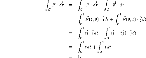
  1. Let's compute the line integral of the vector field tex2html_wrap_inline398 along the curve C which is the straight line from the origin to the point (1,1). One way to describe the curve C is to say it is the graph of the equation y = x as x ranges from 0 to 1. So we can parameterize the line as x = t, y = t, tex2html_wrap_inline418 . Then, we see that, along C, the vector field is tex2html_wrap_inline422 , so

    eqnarray86

  2. Now compute the integral of the same vector field along a new path between the same two points. Let C be made up of two curves, tex2html_wrap_inline426 and tex2html_wrap_inline428 where tex2html_wrap_inline426 is the line segement from the origin to (1,0) and tex2html_wrap_inline428 is the line segment from (1,0) to (1,1). Along tex2html_wrap_inline426 we have tex2html_wrap_inline442 so that tex2html_wrap_inline444 . Along tex2html_wrap_inline428 we have tex2html_wrap_inline448 so that . The line integral is then

    eqnarray98

    Notice that this is the same answer as in the previous example, even though we used a different path of integration. This happened because the vector field is a speacial type of vector field. The entire next chapter will be devoted to studying the interesting properties of these fields, called conservative vector fields. To see that this doesn't always work, try the integrating the vector field over the same two paths.
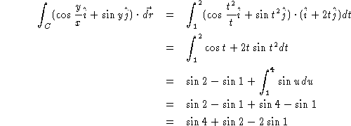
  3. As a final example, consider the vector field tex2html_wrap_inline454 . Compute the line integral of this vector field along the path tex2html_wrap_inline456 between the points (1,1) and (2,4). The proper parameterization of the path is tex2html_wrap_inline462 . Then, tex2html_wrap_inline464 with tex2html_wrap_inline466 .

    eqnarray132


Vector Calculus
Sun Jul 27 11:36:39 MST 1997