
In this section we investigate three interrelated concepts concerning the area under the graph of a function:
In (1) above, we approximate the area under a curve by summing the areas of certain rectangles. The more of these rectangles we use, the more closely their sum approximates the true area under the curve. If we sum an infinite number of these rectangles, we will have the exact area under the curve. In (2) above, we find the antiderivative function f, also called the indefinite integral, denoted by ∫ f′(x)dx, by reversing the rules on the derivative function f′. In (3) above, the Fundamental Theorem of Calculus ties the area under the curve of f′ to its antiderivative f as follows:
That is, the area under the curve y = f′(x) from x = a to x = b, ∫ abf′(x)dx, is the difference of the antiderivative function, i.e. the indefinite integral, evaluated at b and at a. Symbolically, the Fundamental Theorem is written: ∫ abf′(x)dx = f(b) -f(a), where a is called the lower limit of the integral and b is called the upper limit. Another common way of symbolizing the Fundamental Theorem is: ∫ abf(x)dx = F(b) - F(a) where F′ = f. Here F is the antiderivative function of the derivative function f.
We turn now to the procedure for finding the approximate area under a curve. We will illustrate the procedure by taking as our derivative function, f′, a marginal cost function that we will denote by c′(x), where c′(x) is the marginal cost of producing x items of a commodity. We wish to find the area under y = c′(x) from a to b (see the left half of figure 17.1). This area will turn out to be the total variable cost of producing from a to b items of the commodity.
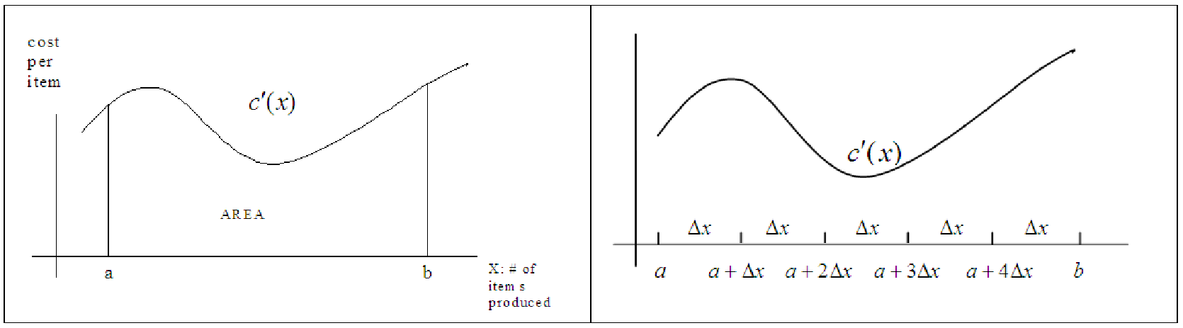
We divide the interval from a to b into n equal subintervals of width (see the right half of figure
?? in which we use 5 subintervals) where Δx =  .
.
For ease of notation, we will rewrite these subintervals as follows: x0 = a, x1 = a + Δx, x2 = a + 2Δx, x3 = a + 3Δx, x4 = a + 4Δx. If we draw a vertical line segment from x = a to the segment’s intersection with the curve (see figure 17.2), the height of this segment represents the marginal cost at a, i.e. the cost of producing one more item when we have already produced a items.
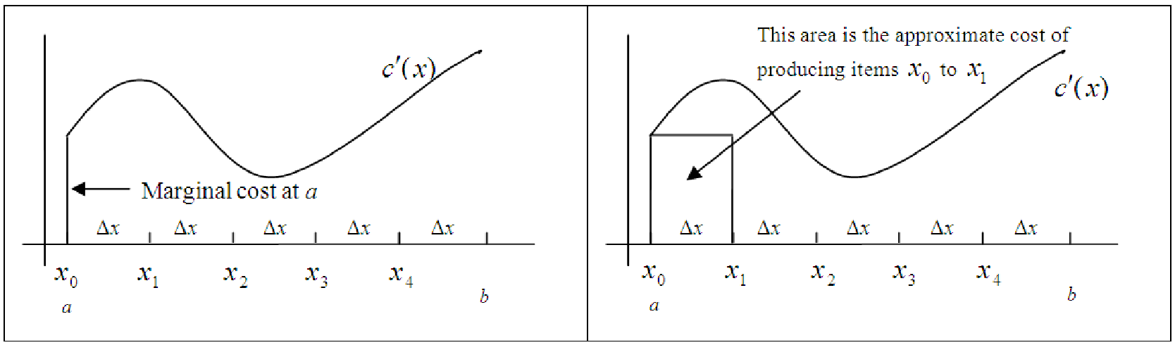
We then create a rectangle with width Δx, the additional items produced beyond a. The area of this rectangle is c′(x)Δx, which is the approximate cost of producing the Δx items from x0 to x1. (See the right half of figure 17.2.)
We will deal with the problem of the area of the rectangle underestimating the true area under the curve from x0 to x1 shortly. Nevertheless, we continue by constructing a second rectangle with a vertical line segment through x1 to the curve c′ with width Δx. The area of this rectangle is the approximate cost of producing items x1 to x2, which happens to overestimate the true area under the curve from x1 to x2 (see Figure 17.5).
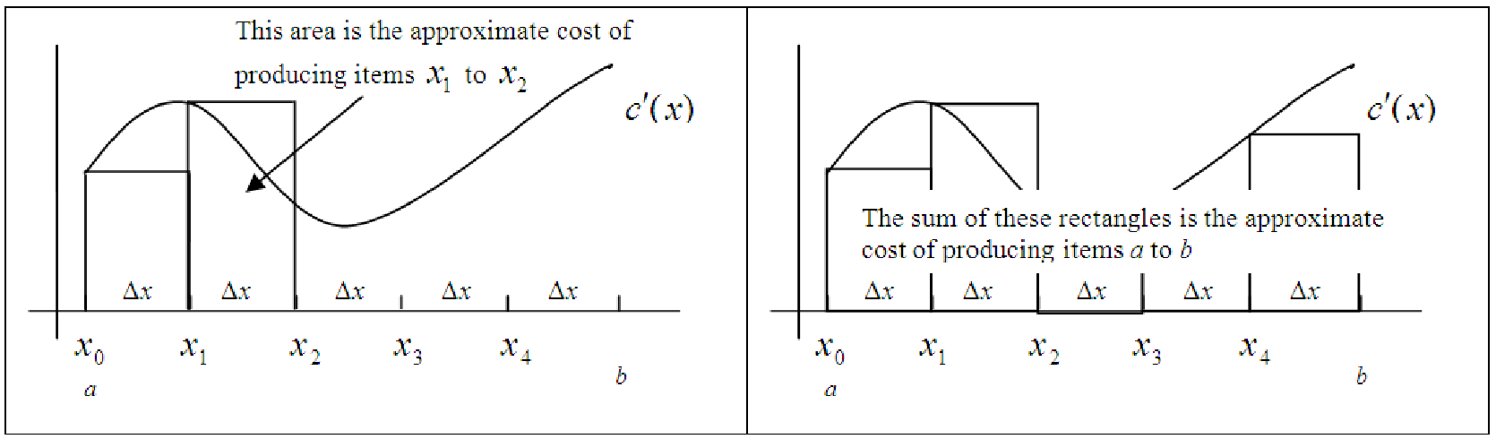
Filling in the remaining rectangles in a similar fashion, we find that the sum of these five rectangles is the approximate area under the curve from a to b (see Figure 17.3).
The approximate area under curve from a to b is

We can imagine constructing an arbitrary number of rectangles n as we have the five above,
each of which has width Δx =  :
:

This is an example of a Riemann Sum (”Rie” rhymes with ”me” and ”mann” rhymes with ”Don.” There are many different ways of constructing rectangles under the curve from a to b, some more accurate and efficient than others. Nonetheless, it turns out that each will lead to the same place, the true area under the curve from a to b. This is how:
We increase the number n of rectangles and correspondingly shrink the width Δx. The over and under estimations of the rectangles decrease as the number of rectangles increases. Mathematically, though not geometrically, it turns out that an infinite number of ”rectangles” can be packed under the curve and summed to give the exact area under the curve from a to b. This is denoted by lim n→∞∑ i=0n-1c′(x i)Δx = ∫ abc′(x)dx and is read ”the limit of the Riemann sum ∑ i=0n-1c′(x i)Δx as n goes to infinity (∞ is the symbol for infinity) is the definite integral of c′(x) from a to b.”