10.2.2 Worked Examples

Example 10.5. Creating and interpreting interaction terms from the EnPact data

An interaction term can be created from a numerical variable and a categorical variable:

We will interpret a rather simple model built on Age, EducLev3 and Age × EducLev3 where EducLev1 indicates a high-school grad and has been chosen as the reference category for the categorical variable EducLev, and EducLev3 indicates a college grad.

Interpretation: When EducLev3 has the value 1, a college graduate is indicated. After substituting 1 for EducLev3 in the model equation, we have

After combing the Age terms, we have a college grad’s salary:

When EducLev3 has the value 0, a high-school graduate is indicated. After substituting 0 for EducLev3 in the model equation, we have

Simplifying, we have a high-school grad’s salary:

Comparing equations (1) and (2), we see that a college grad receives a bonus of $5200 (17.2-12=5.2) for having a college degree plus an additional $220 (.78-.56=.220) for each year that he or she has lived compared to a high-school grad of the same age. At age 30, for example, a high-school grad earns $28,800 whereas a 30-year old college grad earns $40,600. At age 60, they earn $45,600 and $64,000, respectively.

Example 10.6. An interaction terms created from two categorical variables

Suppose we have the variables Gender and EducLev from the previous example, and we plan to construct an interaction term using these variables.

There are 2x5, or 10, interaction terms involved in the interaction variable Gender*Ed. Not all 10 can be submitted to a regression routine, however. Only those interaction terms that do not contain a reference for either variable may be submitted to the regression routine. The following interaction terms are the only ones that may be submitted to a regression routine:

The other interaction terms cannot be submitted to because each contains either one or both of the reference categories (in bold) from which they are created: EdLev1* GenderMale, EducLev1*GenderFemale , EducLev2*GenderMale, EducLev3 * GenderMale, EducLev4 * GenderMale, EducLev5* GenderMale. This means that each of these is a reference category for the interaction variable EducLev*Gender.

We will interpret a modification of the models built above based on the variables Age, EducLev3, Age* EducLev3, GenderFemale and EducLev3*GenderFemale.

Interpretation: If GenderFemale = 0 and EducLev3 = 1, we have a male college graduate. Substituting these values in the model equation, we have

Combining the constants and the Age terms, we have the equation for a male college graduate

If GenderFemale = 1 and EducLev3 = 1, we have a female college graduate. Substituting these values in the model equation, we have

In equation (4) we see that a female receives $4100 more than a male on the basis of gender alone. But she will receive $2500 less than a male if she has a college degree. Simplifying (4), we have the equation for a female college graduate:

Comparing (3) and (5), we see that a female college graduate earns on the average of $1600 (20.4-18.8) more than a male college graduate. The difference is larger, however, for high school graduates (EducLev3 = 0). In this case, female high-school graduates earn $4100 a year more than male graduates. For example, comparing the salaries of 25-year old high school graduates, we have:

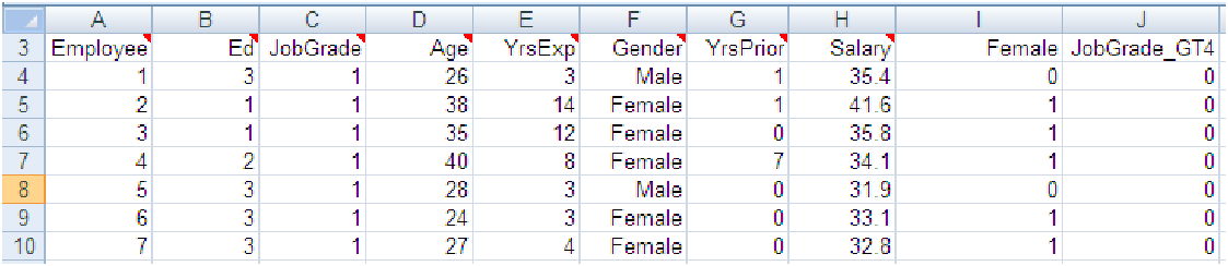
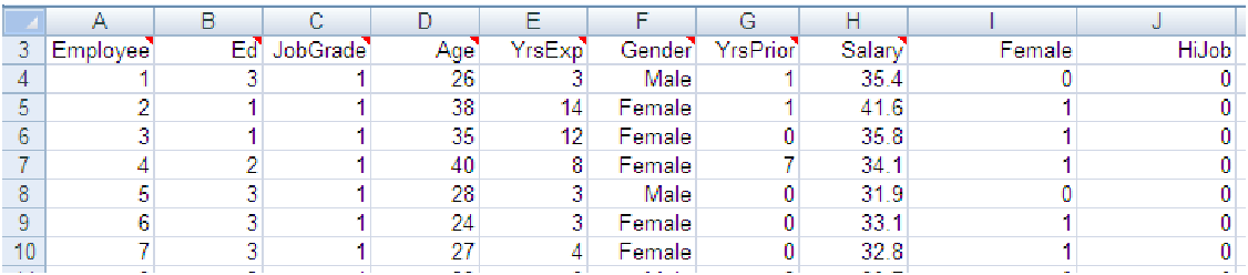
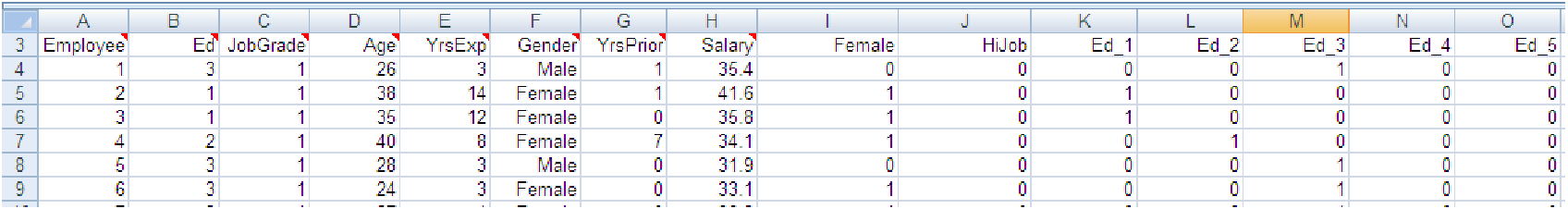
Example 10.7. Simplifying variables in the EnPact data
When we introduce interaction variables into the EnPact gender discrimination study, we find that if we use the given variable names as they are found in C11 EnPact.xls [.rda] the software will create interaction variable names that are too long to be completely viewed in its multiple regression routine window. In addition, when we interact categorical variables with other variables, particularly other categorical variables, the number of possible models from which we must find an optimal model increases greatly, depending on the number of categories involved in creating the interaction terms. There are situations, therefore, in which we have to not only shorten variable names but also combine certain categories together in a meaningful way in order to reduce the number of models we have to analyze. We illustrate how to do this with the EnPact data spreadsheet:

1. Shorten the variable name ”EducLev” to ”Ed” by retyping directly in cell B3
2. At the top of a blank column just to the right of the Salary column, type the variable name ”Female” (do not use quotes). This variable will be a discrete numerical variable with values 0 and 1 to indicate the employee’s gender. If Female has value 1, we have a female employee, whereas if Female has value 0 we have a male. We can do this in Excel by placing the following conditional statement in the first data cell of our new Female variable: =IF(F4=”Female”,1,0). Then we sweep down the column.
3. Generate one categorical/dummy variable based on the categorical variable JobGrade, so that if JobGrade is above 4, the dummy variable is scored as ”True” and otherwise it is ”False” similar to what is shown in figure 10.3. You ay want to simplify the variable names if your software generates long variable names. For example, you could name it ”HiJob” and code it as ”True” or ”False”. HiJob has value 1 (True) if JobGrade is 5 or 6 (this designates a higher level job) and has value 0 (False) if JobGrade is 1, 2, 3, or 4 (this designates a lower job level).
4. Convert ”Ed” to a set of dummy variables, Ed1, Ed2, Ed3, and so forth. See figure 10.5.