Example 16.1. Understanding the optimization problem
We’ll start with a typical sort of optimization problem. Suppose you want to maximize the profit
from selling a variety of products, each of which requires different amounts of different materials
that have different costs. Each of these products has a different demand function and sells for a
different amount of money. As is common, you are required to remain under budget for both
materials and labor.
Suppose our factory makes three products: kitchen tables, kitchen chairs and juice carts. We would like to maximize our profits from selling these three items, given the following information about the price, cost and production time for making each item (each value in the table is given per item produced):
| Item | Assembly time | Finishing time | Materials cost | Selling price |
| Chairs | 1 hr | 1 hr | $5 | $18 |
| Tables | 1 hr. | 4 hr | $15 | $54 |
| Carts | 2 hr | 2 hr | $10 | $36 |
In addition, at our factory we have the following weekly constraints:
| Maximum hours available | Cost per hour | |
| Assembly | 250 hr | $4 |
| Finishing | 350 hr | $7 |
We now need to take this raw information and frame it into a solvable optimization problem.
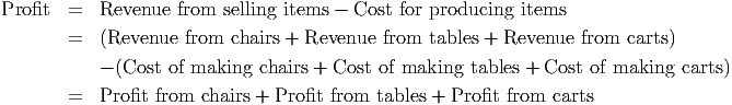
First, what is it we wish to optimize? That would be the profit from selling these items. Thus, the objective function is profit. In this case, the profit is given by the following:
Objective Function (Maximize)
Note that one of our assumptions will be that we sell all of the chairs, tables and carts we make, and that all of these items sell for the listed price.
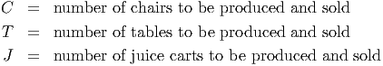
What are the input variables? In this problem, the only things we can change are the number of each item produced. Thus, we have three input variables: the number of chairs produced, the number of tables produced, and the number of juice carts produced. Once we know these numbers, we can compute the total cost for production, the total time for production and the profits we will earn.
What constraints do face? From the given information, it seems that we must keep the total amount of time to produce our chairs, tables, and carts within the amounts listed in the second table. Thus, we have two explicit constraints: the total time for assembly must be less than 250 hrs, and the total time for finishing must be less than 350 hrs.
Constraint #1 (Assembly time <= 200 hr)
Assembly time = chair assembly time + table assembly time + cart assembly time <= 250
Constraint #2 (Finishing time <= 200 hr)
Finishing time = time to finish chairs + time to finish tables + time to finish carts <= 350
At the same time, we have several implicit constraints. These are not stated directly, but are relevant to making sure we have a problem with a sensible solution. Thus, we need to be sure that we produce either zero or a positive number of each product. This gives us the following constraints:
Constraint #3 (Number of chairs produced >= 0)
Constraint #4 (Number of tables produced >= 0)
Constraint #5 (Number of carts produced >= 0)
We have three more implicit constraints: the number of each product that we make and sell must be an integer. After all, we cannot produce and sell one-third of a cart to make one-third of the revenue.
Constraint #6 (Number of chairs produced must be an integer)
Constraint #7 (Number of tables produced must be an integer)
Constraint #8 (Number of carts produced must be an integer)
Thus, even this relatively simple problem leads to eight constraints on the three input variables to maximize a single objective function.
Example 16.2. Mathematizing the optimization problem
Now that we have examined the problem from example 1 and determined the constraints, we can
convert everything into mathematical notation.
Assign names to the variables
The first thing you must do is assign names to the variables. In this case, we will choose the obvious names:
Converting the objective function
To write the objective function as a mathematical expression we need to understand what goes into it. The final form of the profit is probably easiest to work with:
Profit = Profit from chairs + Profit from tables + Profit from juice carts
To determine the profit from selling chairs, we look at four things: the revenue from selling C chairs, the materials cost for making C chairs, the assembly cost for making C chairs and the finishing cost for making C chairs.
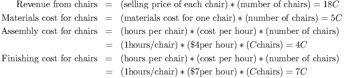
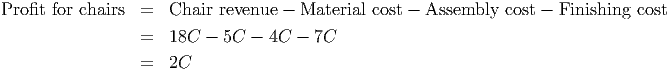
Thus, the profit for making and selling C chairs is
In exactly the same fashion, we compute the following
| Item | Revenue | Material cost | Assembly cost | Finishing cost | Profit |
| Chairs, C | 18C | 5C | 4C | 7C | 2C |
| Tables, T | 54T | 15T | 4T | 28T | 7T |
| Juice carts, J | 36J | 10J | 8J | 14J | 4J |
Thus, the objective function is given by the expression:

Notice that this expression is easy to interpret. For each chair we sell, we earn $2 in profit, for each table we sell, we earn $7 and for each juice cart, $4. In the absence of constraints, the only way to maximize this profit is to make as many of each product as possible. Based on the coefficients, it would seem that making tables is the best way to go. However, that approach would completely ignore the time constraints on making the different products. At 1 hour per table, we could assemble a total of 200 tables. But it would take 200*4 = 800 hours of finishing time to complete those tables. We must keep finishing time below 350, so we can make at most 350/4 = 87.5 tables. But this leaves over half of the assembly hours unused. Perhaps there is some way to make just the right number of each product to use the available resources and increase profits.
Converting the constraints
The constraints on time can easily be converted over. For each chair, we use 1 hour of assembly time. Thus, to make C chairs, we use C hours of assembly time. To make T tables, using 1 hour of assembly time per table, we use up T hours of assembly time. To make J juice carts at 2 hours per cart, we use 2J hours of assembly time.
Constraint #1 (Assembly time <= 250): C + T + 2J <= 250
Similarly, we find the constraint on finishing time:
Constraint #2 (Finishing time <= 350): C + 4T + 2J <= 350
The other constraints are simple to write down, but harder to encode as an expression to be used in doing algebra.
| Constraint #3 (number of chairs >= 0): | C >= 0 |
| Constraint #4 (number of tables >= 0): | T >= 0 |
| Constraint #5 (number of juice carts >= 0): | J >= 0 |
| Constraint #6 (number of chairs is integer): | C integer |
| Constraint #7 (number of tables is integer): | T integer |
| Constraint #8 (number of carts is integer): | J integer |
We have now converted all the expressions into mathematical notation. We could now apply the simplex method or some other technique to solve the problem. Notice that one of the drawbacks to solving the problem this way is that we have all the numbers ”hard coded” into the problem. From the final expressions, it is difficult to see how changing some of the initial information, like the number of hours to assemble a cart or the total number of finishing hours available, will change the expressions without starting over from scratch. In the next section, we will formulate our optimization problems for solution in a spreadsheet. This has the advantage of automatically updating the formulas and expressions based on the new information.
Example 16.3. Minimizing Shipping Costs
CompuTek produces laptops in two cities, Spokane, WS and Atlanta, GA. It purchases screens for
these from a manufacturer, Clear Viewing, that has two production facilities, one located in
Topeka, KS and the other located in Rochester, NY. CompuTek needs these items shipped to its
two facilities. The plant in Topeka can produce at most 2000 units/week, while the plant in
Rochester can produce 1800 units per week. Given the schedule below for how much it costs to
ship a unit of product from each plant to the different cities where CompuTek needs them, how
many should be sent from each plant to each city, if CompuTek needs 1000 units in Spokane and
1200 units in Atlanta?
| Shipping Costs | To
| |
| From | Spokane | Atlanta |
| Topeka | $3 | $2 |
| Rochester | $4 | $5 |
This problem is obviously a minimization problem: we want to keep the shipping costs (our objective function) down to the lowest possible amount. We seem to have four input variables: the amounts shipped from each plant to each final city. And we seem to have two explicit constraints. (1) We cannot ship more from a plant than the plant can produce. (2) We need to ship the right number of units to each city so that CompuTek’s order is filled.
Let’s introduce some variables and express our problem in terms of these variables. We’ll use the following variable names for each of the input variables:
| TS = | the number of units shipped from Topeka to Spokane |
| TA = | the number of units shipped from Topeka to Atlanta |
| RS = | the number of units shipped from Rochester to Spokane |
| RA = | the number of units shipped from Rochester to Atlanta |
| = |
Then, we have the objective function, which is the total shipping cost (TSC):
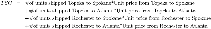
Thus, we see that the total shipping cost is

We want to make this number as small as possible subject to the following constraints:
| We cannot ship more from Topeka than 2000 units: | TS + TA <= 2000 |
| We cannot ship more from Rochester than 1800 units: | RS + RA <= 1800 |
| We need exactly 1000 units in Spokane: | TS + RS = 1000 |
| We need exactly 1200 units in Atlanta: | TA + RA = 1200 |
| All quantities need to be positive: | TA,TS,RA,RS >= 0 |
| All quantities need to be integers: | TA,TS,RA,RS integer |