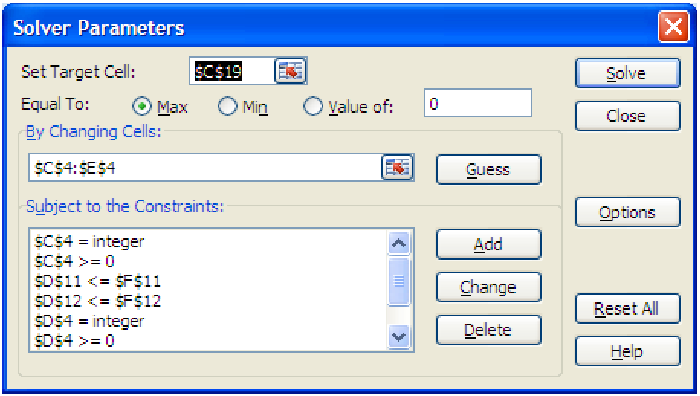
Figure 16.1: Solver dialog box filled in with constraints for solving the furniture problem.
Example 16.4. Solving an optimization problem with Solver Table
In this example, we will actually solve and interpret the results for the production example
described in the last section. We’ll be using file C16 Furniture.xls [.rda]. This relates to the
production of tables, chairs and carts that we set up in examples 1 and 2. For information on how
to set this up in Excel, see the How To Guide for section 16A.
Once the information is entered and the spreadsheet is prepared, you can complete the solution by invoking the solver routine. First, select the cell containing the profit (C19) and then select ”Solver” from the ”Tools” menu. You should get a dialog box like the one below, already set up for you (because the file was saved with this solver scenario already set up). Notice that the first box contains the ”Target Cell” which is our objective function, the profit ($C$19). The next row of information tells solver to maximize the target cell. Notice that you could select ”Min” for minimization problems, or you could set this target cell to a particular value. This last is useful for scenarios of like the one below:
I need to make $700 profit. How many of each product do I need to make?
Problems like this are not, strictly speaking, optimization problems. They are much more like the problems one might use Goal Seek to solve, except solver allows multiple input variables, while Goal Seek only allows one.
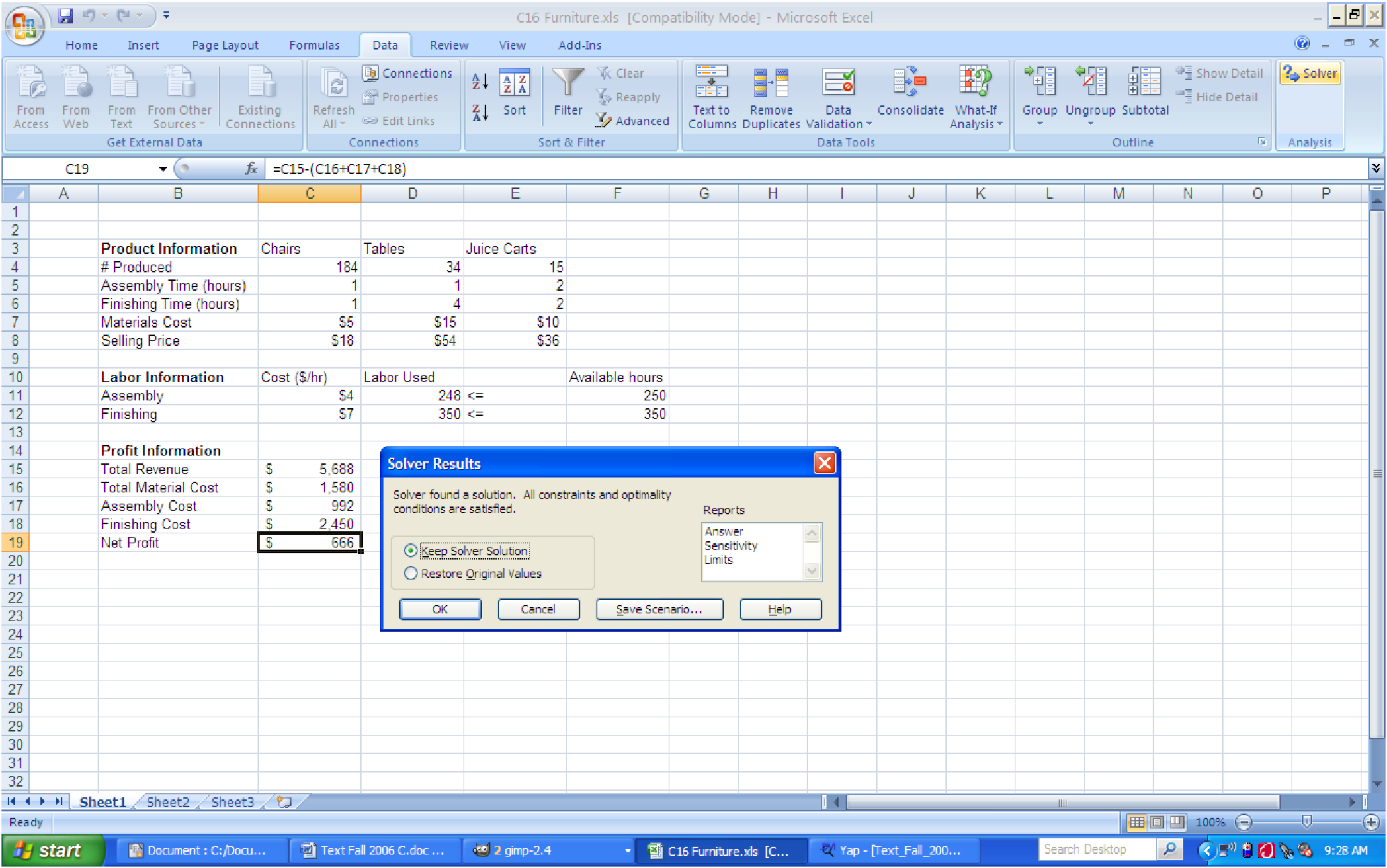
The most difficult part about setting up the solver routine though is the final box, where the constraints are entered. Scrolling down the listed constraints should show you all eight of the constraints identified in example 1. To add another constraint, you simply click the ”Add” button and fill in the dialog box (see the How To Guide for details). Once all the constraints are entered, it can be as simple as hitting the ”Solve” button to get a solution. In this case, solver returns the following screen.
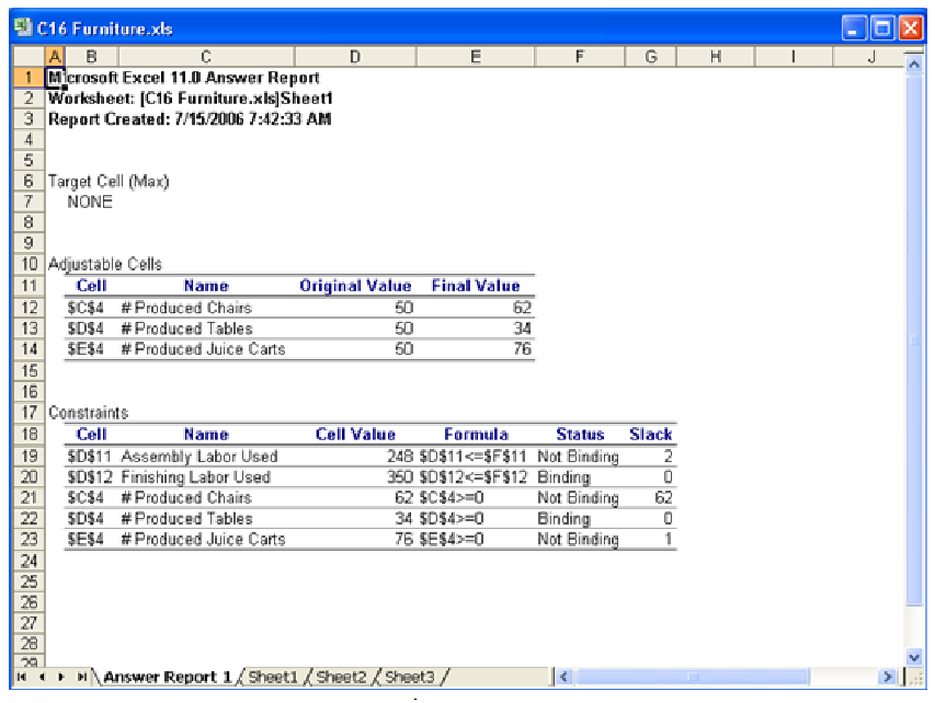
The ”Solver Results” box shows that the routine has found a solution. This solution is displayed in the spreadsheet, and it seems that if we make 62 chairs, 34 tables and 76 juice carts we can maximize our profit at $666. Notice that this solution leaves us with only 2 unused hours of labor (in the assembly area). Clicking on the ”Answer” under ”Reports” and then clicking ”OK” causes solver to create a new sheet (titled ”Answer Report 1”) summarizing the scenario (see the screen below for what this looks like). The report summarizes the initial information and compares this to the final solution. It also summarizes all of the constraints in the problem and whether the constraint was met exactly or whether some ”slack” was allowed.
In this example, we know all of the constraints and the objective function are linear, so we could force Excel to use this information. Clicking on the ”options” button in the solver routine, we can check off the ”Assume Linear” box. Notice, though, that the solution determined in this way is very different from the solution determined otherwise, even though the maximum profit amount, $666, is the same!
We could also have left out the constraints that force the quantity of each product to be positive. Instead, we could have selected the ”Assume non-negative” option in the ”Options” dialog box. The result is the same solution we had originally determined.
Example 16.5. Solving a minimization problem
Let’s solve the problem related to shipping from example 3. We need to organize our
spreadsheet carefully so that we can easily change any of the given information in case
the scenario changes. We also want to set up the spreadsheet so that the calculations
are easy to copy. The screen shot below shows how we have chosen to organize the
information.
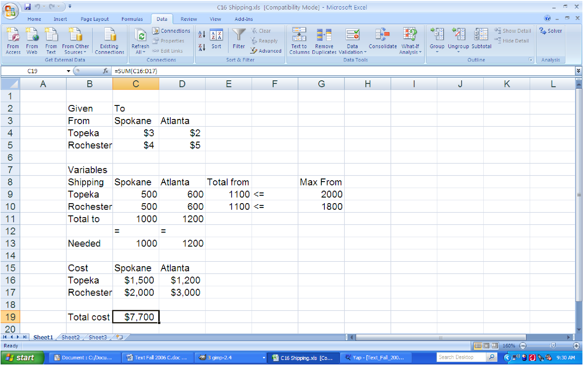
Notice that the given information about the shipping costs from each plant to the final cities is listed at the top (cells B3:D5), and they are organized into a table much like the one that originally stated the information. This structure will be repeated throughout the setup of this problem. Below that, we have the temporary values for our input variables. These are also organized into a table in cells B8:D10. To the right of the variables are some calculations. Cell E9 contains the total number of units shipped from Topeka (=C9+D9), which is then copied to cell E10 to get the number of units shipped from Rochester. Cells F9:F10 contain symbols to remind us what the constraints are (¡=) and G9:G10 contain the maximum number of units that can be shipped from the two plants. Below the variables, in cells B12:D13, we have information about the number of units needed in each city.
The next table, cells B15:D17 contains calculations for the total cost of shipping from each plant to each city. For example, in cell C16, the formula ”=C9*C4” has been entered; this computes the cost for shipping a total of C9 units from Topeka to Spokane at a cost of C4 dollars per unit. This formula can then be directly copied to the other cells in the table to compute the corresponding amounts of shipping from each plant to each city.
The final piece of the setup is in cell C19: the total shipping cost. This is simply the formula
”=SUM(C16:D17)”. This will be the objective function that we minimize.
Selecting C19 and invoking the solver routine, we make sure to select ”minimize” and then we enter our four input variable, found in cells $C$9:$D$10. There are three constraints:
| Constraint | Notation in Solver |
| Total Shipped <= Maximum Output | $E$9:$E$10 <= $G$9:$G$10 |
| Total Received = Total Needed | $C$11:$D$11 = $C$13:$D$13 |
| All amounts are integers | $C$9:$D$10 integer |
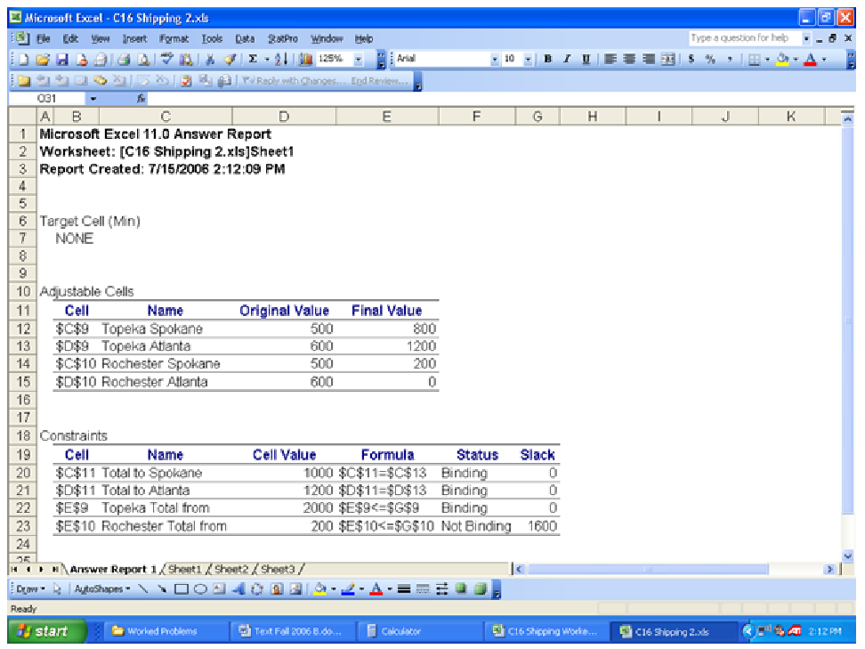
Then, we set the options for the solver routine so that ”Assume non-negative” is checked, and solve the problem. The answer report from the solver routine is shown below. It seems we should TS = 800, TA = 1200, RS = 200, and RA = 0.
Example 16.6. Special case - two input variables and one constraint
In some situations, optimization problems for multivariable functions are much easier to solve. One
of these situations, one that occurs frequently, is when your objective function has two input
variables and only one constraint function. In principle, any problem of this kind can be converting
into a single variable optimization problem like those solved in chapter 14. Let’s see how this
works.
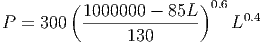
Consider a typical model of production for an economy using a Cobb-Douglas (multiplicative) model like the one below. The two input variables are K, the units of capital invested in the economy, and L, the units of labor invested in the economy.

In most situations, we would like to maximize the productivity of the economy by setting the labor and capital investments appropriately. Thus, the productivity becomes our objective function. But we cannot choose just any values for K and L. Suppose that each unit of labor costs 85 and each unit of capital costs 130. If costs must be maintained below 100,000, then we want to maximize the productivity above, subject to the constraint that
Total Cost = 130K + 85L <= 100, 000
Notice that for the type of function we have we can increase the objective function by making the input variables as large as possible. This, and other obvious logic, lead us to conclude that the only place we will get a solution to this problem is if the total cost is exactly equal to its maximum value, 100,000. (If we went for less, then another unit of capital or labor would push the cost closer to the maximum possible cost and would increase the productivity of the economy.) This means that we will take the constraint to hold at equality. That gives us a linear equation, which we can solve for one of the two variables:

If we plug this value of K into the objective function, we get
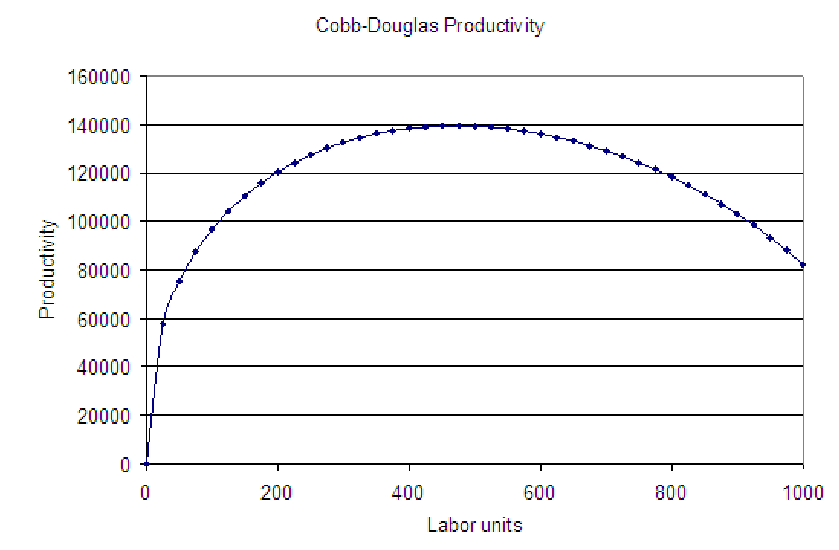
This is a function of one variable! We can graph it easily and estimate the value of L for which the productivity, P, is maximum. We can then plug this value of L into the equation for K to find the number of units of capital we need to reach maximum productivity. The graph is shown below, indicating that about 500 units of labor are needed. Using the methods from chapter 14, we find that a better estimate is 470.59 units of labor. This results in 461.53 units of capital needed to achieve maximum productivity.
We could also solve this by setting the derivative of the production function to zero with Goal Seek. Computing the derivative of the objective function (after substituting in the constraint) will require the product rule and the chain rule.