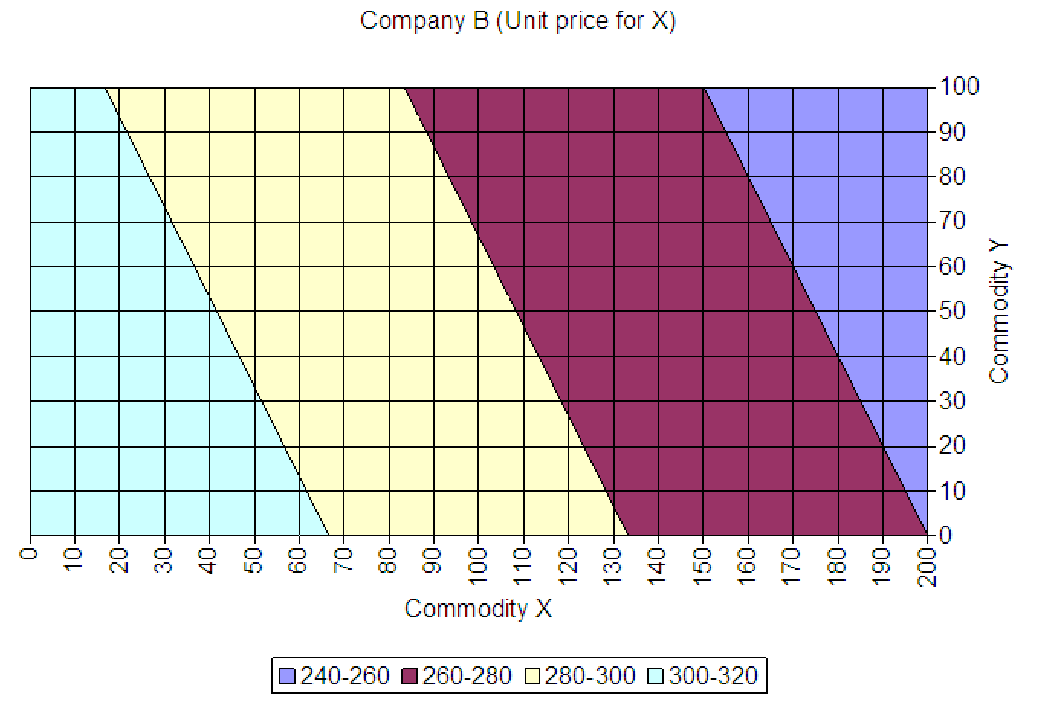
Figure 13.12: Contour plot of demand function for Company A in problem 6.
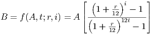
13.6. The graphs below show contour plots of the demand function for one product out of a pair of products sold by the same company. In each graph, the demand function plots the unit price when x and y units of the two products are demanded. Which company is selling two complementary commodities? Which is selling two substitute commodities? Explain your answer.
13.7. Metro Area Trucking has been gathering data regarding a different approach to predicting maintenance costs of its trucking fleet. There is a considerable growing body of research suggesting than uneven tire tread wear is related to maintenance costs for a variety of reasons including worn front end parts, worn or weak suspension, and even the vibrations of a roughly running engine. The surface of the roadway has been shown to affect uneven tire wear, which might relate to maintenance costs even apart from tire wear, and uneven tire wear is a direct contributor to high gasoline costs. Metro has developed an index for measuring uneven tire wear. Every three months the treads of the four tires of a van are each measured in three places by a digital gauge to the nearest 64th of an inch. The standard deviation of the three measurements taken on each tire is calculated and then scaled from 1 to 100 in whole numbers for easy reading. This is called the tire’s tread index. The more uneven a tire is, the larger its standard deviation, and the higher its tread index. The largest index measured from the four tires on the van is recorded. The idea is that this index, which is a measure of the driving conditions to which the truck is subjected, interacted with the number of miles the truck is driven, might very well be a good predictor of maintenance cost.
13.8. Consider the following model to explain the number of tickets sold each week in a large metro public transportation system:

In this model, the variable ”Income” represents average weekly disposable income for a family of four in the greater metropolitan area (in dollars), ”TicketPrice” represents the price of a ticket on the transit system (in dollars), and ”Gas Price” is the median price for a gallon of regular unleaded gas (in dollars).
But the model, with three variables, is too complicated for explaining to the city council at the upcoming meeting. You have noticed that, within the time span that this model was based upon, you found that

Use this information to find a simpler way to express the model and interpret the simplified model both algebraically and graphically.
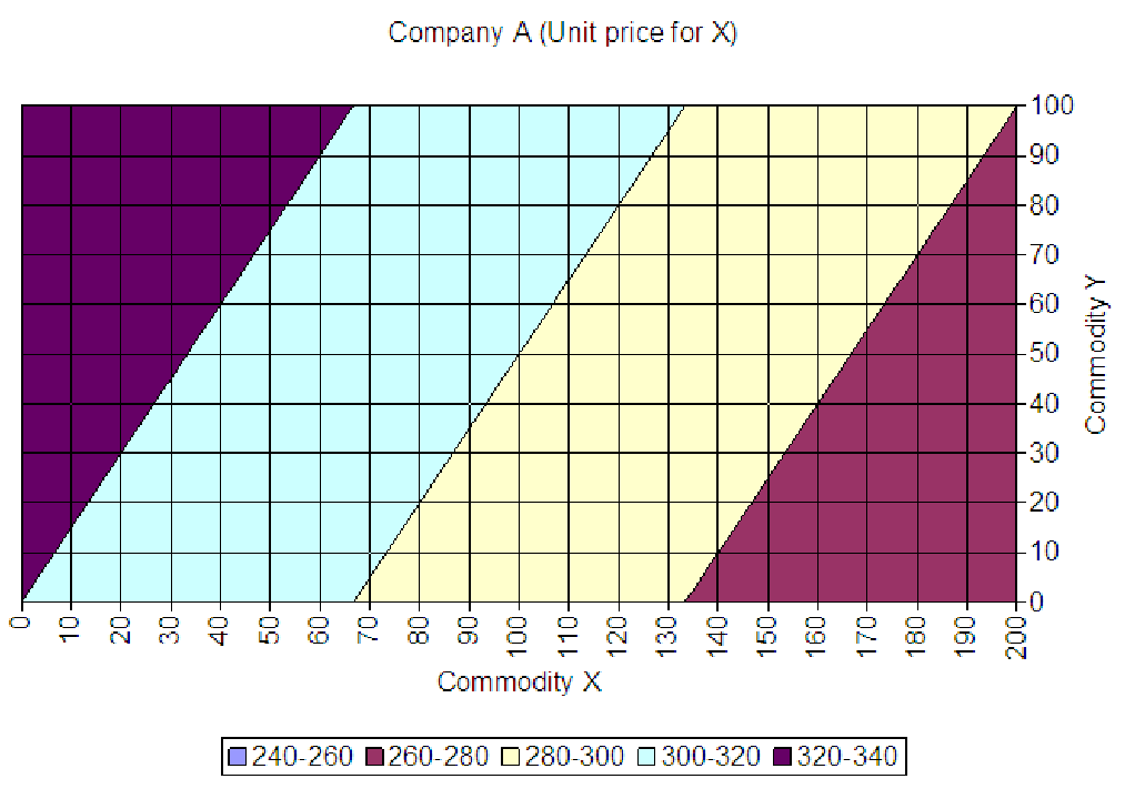
13.9. For a fixed amount of principal, A (in dollars), the monthly payment ($) for a loan of t years at a fixed APR of r is given by the formula below.
![Ar
P = f(A; r,t) = --[----(------)--12t]-
12 1 - 1 + -r
12](Text_Fall_2014247x.png)
13.10. Home mortgage rates are designed so that the amount of principal and amount of interest in each payment varies over the life of the loan, but the monthly payment remains fixed. For a loan of A dollars and a term of t years, the total amount of principal paid by the end of month i of the loan is given by the formula below.