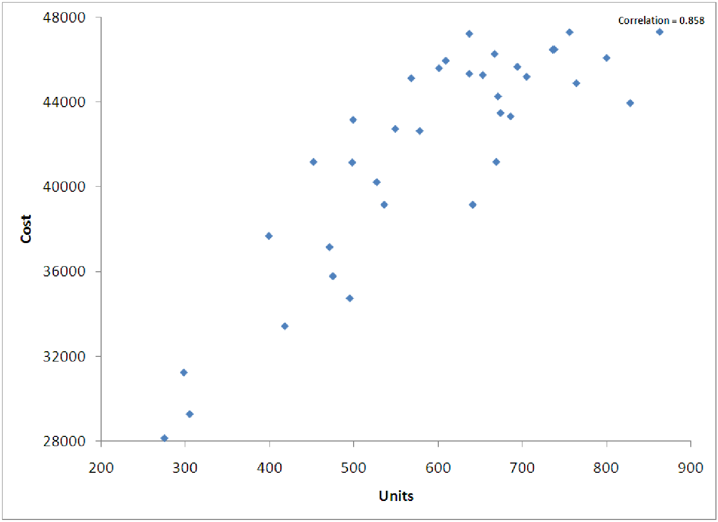
Figure 12.1: Graph of electricity cost vs. units of electricity.
To perform nonlinear regression, we have to ”trick” the computer. All the regression routines in the world are essentially built on the idea of using linear regression. This means that we must find a way to ”linearize” the data when it is non-proportional. Consider the data shown in figure 12.1. It represents the cost of electricity based on the number of units of electricity produced in a given month. The relationship is obviously in the shape of a logarithmic function.
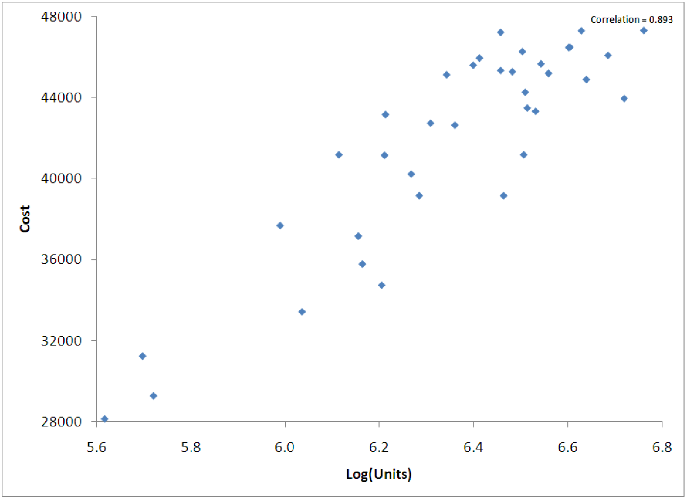
Since the relationship indicates a logarithmic relationship, we examine, in figure 12.2, a graph of Cost vs. Log(Unit). Notice that this graph is ”straighter”, indicating that we could use linear regression to predict Cost as a function of Log(Units). Thus, we can ”trick” the computer into using linear regression on nonlinear data if we first ”straighten out” the data in an appropriate way. An explanation of the straightening out process can be found in example 5.
Another way to say this is that the relationship is linear, but it is linear in Log(x) rather than linear in x itself. Thus, we are looking for an equation of the form y = A + B log(x) rather than an equation of the form y = A + Bx. Notice that we are free to transform either the x or the y data or both. These different combinations allow us to construct many different models of nonlinear data.
We can also perform nonlinear analyses on data with more than one independent variable. In most cases, though, the only appropriate model for such data is a multivariable power model, called a multiplicative model. Such models are used mainly in production and economic examples. A famous example is the Cobb-Douglas production model which predicts the quantity of production as a function of both the capital investment at the company and the labor investment. See the examples for more information.
In the rest of this section, we’ll talk about how to select and complete the appropriate transformations, how to use these in regression routines, and how to compute R2 and S e in certain cases.