Figure 12.3: Plot of residuals versus fitted values for a linear model of predicting production
vs. labor and cost.
Example 12.1. One independent variable example (X transform)
The electricity data shown above (see figures 11.A.1 and 11.A.2 and the data file C12 Power.xls
[.rda]) seems to be linear in either square root(units) or log(units) rather than linear in
units. This means that we can construct a model for the cost of the electricity that
is linear in either square root(units) or log(units). This model will look like Cost =
A + Bx.
However, the x in this case will be either square root(units) or log(units) rather than units. To construct the models, we start by creating new variables in the data called ”sqrt(units)” and ”log(units)”. For example, StatPro allows you to do this automatically through the ”Data Utilities/ Transform Variables” function, and R Commander allows you to do this through the ”Data/Manage variables in active data set... ” menu. Once we have these new variables, we then go through the normal regression routines, using ”Cost” as the response variable and either ”Sqrt(units)” or ”Log(units)” as the explanatory variable. The result of the regression routine when using sqrt(units) is shown below.
| Results of multiple regression for Cost
| |||||||
|
| |||||||
| Summary measures | |||||||
|
| Multiple R | 0.8786 | |||||
|
| R-Square | 0.7719 | |||||
|
| Adj R-Square | 0.7652 | |||||
|
| StErr of Est | 2540.5818 | |||||
|
| |||||||
| ANOVA table | |||||||
|
| Source | df | SS | MS | F | p-value | |
|
| Explained | 1 | 742724176 | 745724176 | 115.0698 | 0.0000 | |
|
| Unexplained | 34 | 219454912 | 6454556 | |||
|
| |||||||
| Regression coefficients | |||||||
|
| Lower | Upper | |||||
|
| Coefficient | Std Err | t-value | p-value | limit | limit | |
|
| Constant | 6772.5645 | 3290.6382 | 2.0581 | 0.0473 | 85.1875 | 13459.94 |
|
| Sqrt(Units) | 1448.7365 | 135.0544 | 10.7271 | 0.0000 | 1174.2730 | 1723.19 |
This leads us to the first nonlinear model for this data:
Cost = 6,772.56 + 1,448.74*Sqrt(units).
This model is linear in square root(units). We can perform the same technique using the log(units) variable. The output from the regression routine is shown below and leads us to the model equation:
Cost = -63,993.30 + 16,653.55*Log(Units).
This model is logarithmic in units; it is also said to be linear in log(units). This idea that the model is linear in a transformed variable is how we ”trick” the computer into creating non-proportional models by performing linear regression. Notice that the logarithmic model is slightly better (it has a lower standard error) but the constant term is negative, making interpretation of this model more difficult.
| Results of multiple regression for Cost
| |||||||
|
| |||||||
| Summary measures | |||||||
|
| Multiple R | 0.8931 | |||||
|
| R-Square | 0.7977 | |||||
|
| Adj R-Square | 0.7917 | |||||
|
| StErr of Est | 2392.8335 | |||||
|
| |||||||
| ANOVA table | |||||||
|
| Source | df | SS | MS | F | p-value | |
|
| Explained | 1 | 7.68E08 | 7.67E08 | 134.0471 | 0.0000 | |
|
| Unexplained | 34 | 1.95E08 | 5.23E06 | |||
|
| |||||||
| Regression coefficients | |||||||
|
| Lower | Upper | |||||
|
| Coefficient | Std Err | t-value | p-value | limit | limit | |
|
| Constant | -63993.3047 | 9144.3428 | -6.9981 | 0.0000 | -82576.8329 | -45409.78 |
|
| Log(Units) | 16653.5527 | 1438.3953 | 11.5779 | 0.0000 | 13730.3838 | 19576.82 |
Example 12.2. Another one independent variable example (Y transform)
Consider again the data in C13 Power.xls [.rda]. Suppose we decide to construct a power
function fit for the data. Basically, a power model is a model in which the log(response) variable is
linear in the log(explanatory) variable. Thus, we seek a model of the form
Log(Cost) = A + B*Log(Units).
For this, we first create variables log(cost) and log(units). We then perform the standard linear regression, using Log(cost) as the response and log(units) as the explanatory. The result is shown below. N.B. The summary measures are completely useless for this type of model, since they are all based on Log(Cost) rather than actual cost. We must compute the correct summary measures for ourselves (see the How To Guide of this section for an example and the steps.) The actual correct summary measures are R2 = 0.7736 and S e = 2530. These are slightly better than the results of the linear fit (R2 = 0.7359, S e = 2733.)
| Results of multiple regression for Log(Cost)
| |||||||
|
| |||||||
| Summary measures | |||||||
|
| Multiple R | 0.8967 | |||||
|
| R-Square | 0.8040 | |||||
|
| Adj R-Square | 0.7983 | |||||
|
| StErr of Est | 0.0617 | |||||
|
| |||||||
| ANOVA table | |||||||
|
| Source | df | SS | MS | F | p-value | |
|
| Explained | 1 | 0.5312 | 0.5312 | 139.4835 | 0.0000 | |
|
| Unexplained | 34 | 0.1295 | 0.0038 | |||
|
| |||||||
| Regression coefficients | |||||||
|
| Lower | Upper | |||||
|
| Coefficient | Std Err | t-value | p-value | limit | limit | |
|
| Constant | 7.8488 | 0.2358 | 33.2797 | 0.0000 | 7.3695 | 8.3281 |
|
| Log(Units) | 0.4381 | 0.0371 | 11.8103 | 0.0000 | 0.3627 | 0.5135 |
Example 12.3. The Multiplicative model
Consider the data shown in file C12 Production.xls [.rda]. This data shows the total production
of the US economy (in standardized units so that it is 100 in 1899) as well as the investment in
capital (K, also standardized) and labor (L, also standardized). We want to construct a model for
predicting the productivity as a function of the capital and labor. We basically take two
approaches with such multivariable data:
Approach 1. Try a multiple linear model.
Approach 2. If the linear model doesn’t work well, try a multiplicative model.
Approach 1 in action. First we try predicting P as a linear function of K and L. (This is just like multiple linear regression models that we have seen before, so we omit some details.) The resulting model and summary measures are shown below.
P = -2 + 0.8723L + 0.1687K
R2 = 0.9409
Se = 11.1293
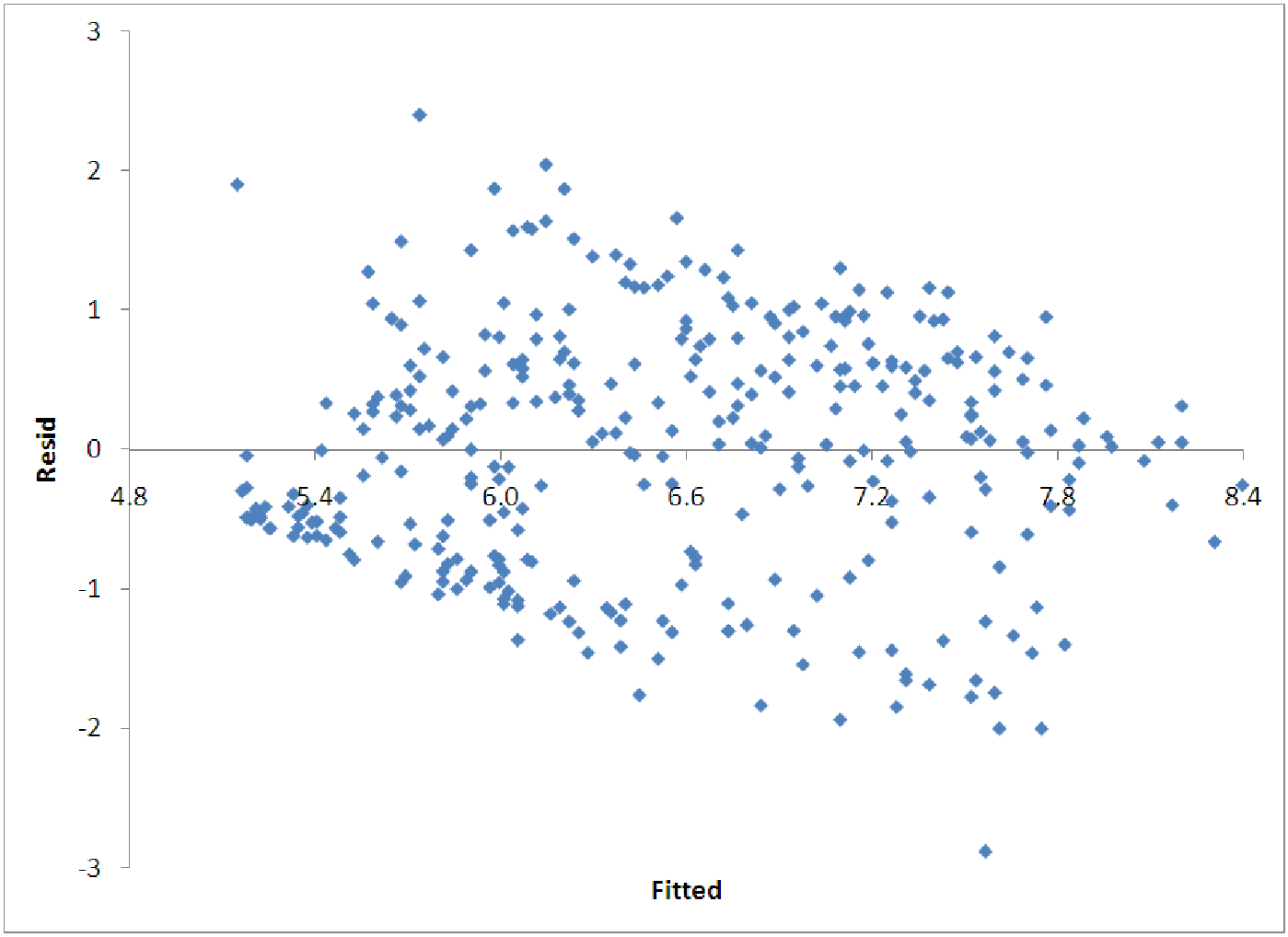
Thus, it seems that a linear model does quite well, based on this information. However, in examining the diagnostic graphs, we notice that the residuals seem to spread out. To correct this, we try logging all the variables and producing a multiplicative model.
Approach 2 in action. So, now we transform each of the variables using the logarithmic transformation. This produces three new variables - log(P), log(K) and log(L). We then perform a multivariable regression on log(P) as a function of both log(K) and log(L) to get the following results. Notice that we have computed the actual R2 and S e values using the techniques described in the computer how to for this section. Since we have logged the response variable (P) we cannot believe the regression output values for the summary measures.
log(P) = -0.0692 + 0.7689 log(L) + 0.2471 log(K)
R2 = 0.9386
Se = 11.3449
This model has about the same explanatory power as the linear model (very high, both are above 90% for R2.) Furthermore, we notice that the patterns in the residuals are no longer apparent. Interpreting this model will be left to the next section, but note that we can, with a little algebra, convert the model equation into the familiar form for a Cobb-Douglas production model. The result is P = 0.9331L0.7689K0.2471. Such models play an important role in many economic settings.
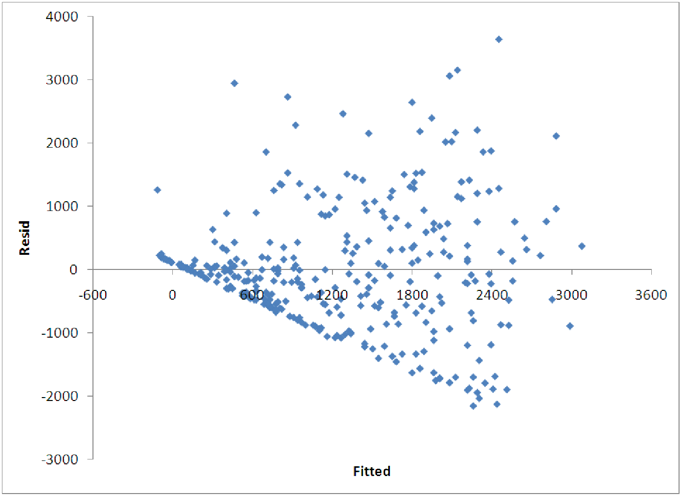
Example 12.4. Non-constant variance
The data in file C12 Baseball.xls [.rda] shows the salaries of over 300 major league
baseball players along with many of their statistics for a particular season. Suppose
that we want to predict the salary of a player based on the number of hits the player
had during the season in order to test the assumption that better players have higher
salaries.
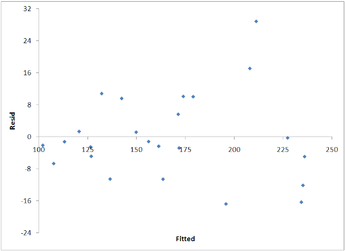
If we do this, we see that the model is not very accurate (R2 = 0.34). The reason for this is apparent in the plot of the residuals versus the fitted values (figure 12.4). One clearly sees the fan shape of these residuals, indicating that higher salaries also have higher variation from the model predictions.
To handle a fan that opens to the right, we typically log the response variable. Thus, we look for a model of the form log(y) = A + Bx. Transforming the response variable produces the model equation log(Salary) = 5.1305 + 0.0151*Hits. This model has the pattern for the residuals shown above in figure 12.5. Notice that the non-constant variance is greatly reduced. There does remain some narrowing of the pattern on the left, but this is largely due to the fact that there is a minimum salary in the data, so that there are no observations with actual salaries below a certain level.
It is also possible for the residuals to fan in the opposite pattern: spread out on the left and narrowing to the right. If this is the case with the data, we typically use the reciprocal of the response variable in the model.
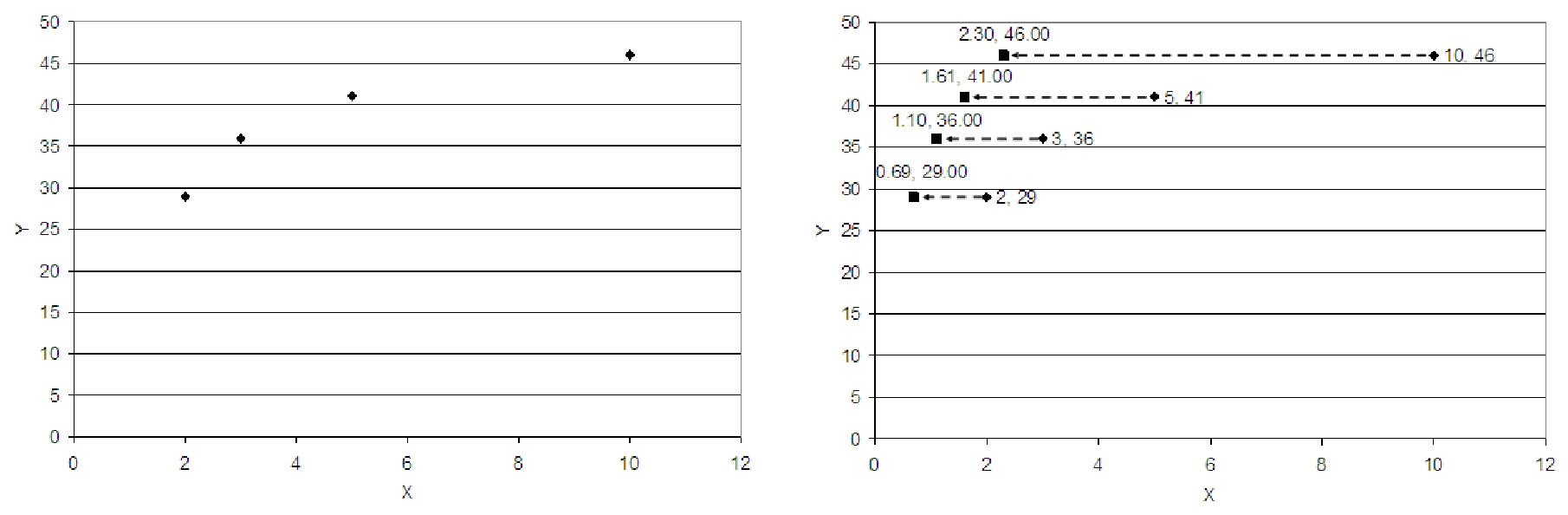
Example 12.5. Straightening out data
The two graphs below show how the logarithmic function can be used to straighten out data that
is non-proportional. In figure 12.6, we see data (indicated by the diamond shapes) that does not
appear to be linear. These data have the coordinates (xi,yi). To straighten the data out, we plot y
versus the natural log of each of the x coordinates using squares to indicate these points in figure
12.7. Thus, we see how the original data points (xi,yi) are transformed to the data (ln(xi),yi)
which have a less extreme curve.