
Example 6.1. Estimating the mean
Suppose we have been presented with a table of information like that below which summarizes the
salaries of the employees at a company. What is the average salary at your company (as
determined by using the mean)?
| Salary Range | Number of Employees |
| $200,000 - $250,000 | 1 |
| $150,000 - $199,999 | 2 |
| $100,000 - $149,999 | 5 |
| $50,000 - $99,999 | 13 |
| $0 - $49,999 | 38 |
We notice several problems immediately. First, we do not have the actual salaries of each employee; we only know a range of salaries. Second, each employee in each range could have a different salary within that range. How can we compensate for this?
The first problem is one of identifying a particular salary to represent each range. Common choices are the midpoint of the range and either endpoint. We will start with the midpoint and then repeat the analysis using the endpoints. The second problem is more interesting. Typically, we assume that all the observations in a given range of salaries are the same. Clearly, this is a poor assumption, but without it we cannot really get anywhere. This ambiguity in dealing with summarized data is why we can only claim to be estimating the mean of the data, not computing it. Based on these assumptions, we now have the following table of data to work with (after rounding the salaries off).
| Salary | Number of Employees |
| $225,000 | 1 |
| $175,000 | 2 |
| $125,000 | 6 |
| $75,000 | 13 |
| $25,000 | 38 |
So, is the average just (225,000 + 175,000 + 125,000 + 75,000 + 25,000)/5 = $125,000? That would seem to be a bit high, wouldn’t it, since only 8 employees make that much money and 51 employees are below that level. The problem with this kind of computation is that each of the salary ranges must be weighted. This means that we must put several copies of each salary into the calculation, one copy for each observation that matches that data value. Think about it this way, if we had a complete list of the salaries for computing the mean, it would look something like the table below.
| 225,000 | 75,000 | 75,000 | 25,000 | 25,000 | 25,000 |
| 175,000 | 75,000 | 75,000 | 25,000 | 25,000 | 25,000 |
| 175,000 | 75,000 | 25,000 | 25,000 | 25,000 | 25,000 |
| 125,000 | 75,000 | 25,000 | 25,000 | 25,000 | 25,000 |
| 125,000 | 75,000 | 25,000 | 25,000 | 25,000 | 25,000 |
| 125,000 | 75,000 | 25,000 | 25,000 | 25,000 | 25,000 |
| 125,000 | 75,000 | 25,000 | 25,000 | 25,000 | 25,000 |
| 125,000 | 75,000 | 25,000 | 25,000 | 25,000 | 25,000 |
| 125,000 | 75,000 | 25,000 | 25,000 | 25,000 | 25,000 |
| 75,000 | 75,000 | 25,000 | 25,000 | 25,000 | |
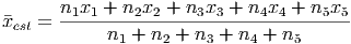
To add up all these salaries and compute the mean, we would need to include 2 copies of the $175,000 salary, 6 copies of the $125,000 salary and so on. Thus, we estimate the mean (measuring the data in thousands of dollars) as
Clearly this number is more reasonable for the salary. How can we estimate such means in general? First, we need to assign symbols to each quantity. Suppose we have N different groups of data. In the above example, we have 5 groups of data, so N = 5. Let the value of the ith range be (where ) and we will let the number of data points in the ith range be given by . With these naming conventions, the data table above would look like this:
| Salary | Number of Employees | Product |
| xi | ni | xini |
| x1 = $225,000 | n1 = 1 | 225,000 |
| x2 = $175,000 | n2 = 2 | 350,000 |
| x3 = $125,000 | n3 = 6 | 750,000 |
| x4 = $75,000 | n4 = 13 | 975,000 |
| x5 = $25,000 | n5 = 38 | 950,000 |
| Total | 60 | 3,300,000 |
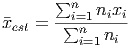
Now, to compute the mean, we multiply each data value (the x’s) by its weight (the n’s) and add these up. Then we divide by the total number of observations (the sum of all the n’s):
Using the sigma notation, this becomes much easier to write down:
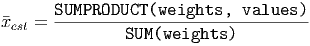
Now, if we’re using Excel, the numerator can be computed as a ”sum product” (or vector dot product) of two lists of numbers. One is the list of weights and the other is the list of the values associated with the data ranges. Using this, we can write the Excel version of the weighted average formula as
Example 6.2. Effects of different midpoints
Using example the previous example, we can compute the average is several different ways, using
different values for the data range. Below is a table showing the estimation of the mean for the
salary data above, using the midpoint, left endpoint and right endpoint of each range of values.
Keep in mind, though, that unless you have a very good reason for doing otherwise, you
should probably use the midpoint to estimate the mean, since that will likely be a better
representation of the data in any particular bin. Using the endpoints implies that the
data within a particular bin is highly skewed, which might be the case, but would need
justification.
| Salary Range | Number of employees | Midpoint | Left | Right |
| $200,000 - $249,999 | 1 | 225,000 | 200,000 | 249,999 |
| $150,000 - $199,999 | 2 | 175,000 | 150,000 | 199,999 |
| $100,000 - $149,999 | 6 | 125,000 | 100,000 | 149,999 |
| $50,000 - $99,999 | 13 | 75,000 | 50,000 | 99,999 |
| $0 - $49,999 | 38 | 25,000 | 0 | 49,999 |
| Estimated Average | $54,166.67 | $29,166.67 | $79,165.67 | |
As you can see, the choice of where to place the value for each data range has a huge effect on the estimate of the mean. In fact, if each of the ranges has the same degree of spread (all of the ranges above cover $49,999) the estimate of the mean from the left and right endpoints will differ by the spread (notice that $79,165.67 - $29,166.67 = $49,999, the spread of the data in each of the ranges). Mathematically, this is easy to prove. Assume that each range has a spread of S. Then, if the left endpoints of the ranges are given by xi, the right endpoints are given by xi + S and the estimate for the mean using the right endpoint will be (all sums are from i = 1 to i = n)

However, there is any easier way to see what happens using different estimates for the data points. Recall that if we add the same amount to every single data point it will shift the mean by that amount exactly. So if we add 10 to each data point, the mean will increase by 10.
Thus, with summarized data, we can never nail down an exact value for the mean. At best, we can estimate it to fall within a particular span of values that is closely tied to the spread each range of data covers.
Example 6.3. Averaging Averages
We can also use the previous examples to understand why we cannot average several averages:
Each average must be weighted by the number of data points used to compute that average. For
example, if we have two sections of a course being taught and the two sections take the exact same
final examination, we might want to determine the overall average on the final exam before
deciding what grades to give. If one class scored an average of 82 on the final exam and the
other class scored an average of 75 on the final, we cannot simply say that the overall
average is (82 + 75)/2 = 78.5 because the two classes may have very different numbers of
students. The table below uses the correct method, weighted averages, to determine the
overall average for different sizes of each class. Notice that the more students there are in
the class with the high average, the closer the overall average is to that class’s average
score.
| Class 1 Size | Class 2 Size | |
| (test ave = 82) | (test ave = 75) | Overall Average |
| 10 | 30 | 76.75 |
| 15 | 15 | 78.5 |
| 30 | 10 | 80.25 |
| 35 | 5 | 81.125 |
Also note that when averaging averages, we are not estimating the mean; in this case we are computing the actual mean of the combined data. Algebraically, we can see why. To compute the weighted average in the above case, the numerator will be n11 + n22, but when we multiply an average by the count of data points (the n) we are getting the actual total of all the data points, since
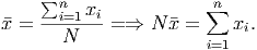
So in this case, the numerator is the exact total of all the data points in each class, even though we do not have the individual scores for any particular student!
Example 6.4. Estimating Standard Deviation
Estimating the standard deviation for summarized data is not that much different from calculating
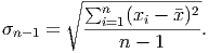
the standard deviation normally. Recall that the formula for the sample standard deviation of a set
of data given by x1,x2,…,xn is simply
When we only have a summary of the data, though, we must estimate the data points and then weight the deviations based on the number of data points falling near that estimated value. Thus, the formula becomes
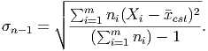
where we have used the symbol Xi to refer to the estimate of the value of the data in the ith bin of the summarized data, ni is the number of data points in that bin, and m is the total number of bins in the summary.
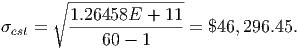
Using the data from the previous section, we can compute each piece of the formula and combine them into an estimate of the standard deviation in the salaries. We will use the midpoint estimate for both the mean and the standard deviation. Recall that the estimate for the mean salary was $54,166.67.
So, the estimate for the standard deviation is
| Salary | Number of | Midpoint | Deviation | ni(Xi -est)2 |
| Range | employees (ni) | (Xi) | (Xi -est) | |
| $200,000 - $249,999 | 1 | 225,000 | 170,833 | 29184027778 |
| $150,000 - $199,999 | 2 | 175,000 | 120,833 | 29201388889 |
| $100,000 - $149,999 | 6 | 125,000 | 70,833 | 30104166667 |
| $50,000 - $99,999 | 13 | 75,000 | 20,833 | 5642361111 |
| $0 - $49,999 | 38 | 25,000 | -29,167 | 32326388889 |
| Sum | 60 | 1.26458E+11 | ||
Computing the quartiles for this data is relatively easy. Since there are 60 data points, each quartile should contain 15 points (60/4 = 15). Thus, starting at the smallest value, the first quartile is between the 15th and 16th data points. This would place the first quartile in the first bin, between $0 and $49,999. The second quartile would fall between the 30th and 31st data points, also in the first bin. The third quartile would lie between the 45th and 46th data points, placing it inside the second bin, between $50,000 and $99,999. Our estimates of the statistics relating to this data are then gathered together below.
| Mean | 54,166.67 |
| Standard deviation | 46,296.45 |
| Q1 | 25,000 |
| Q2 = median | 25,000 |
| Q3 | 75,000 |
With summarized data, this is about as accurately as one can estimate the standard deviation and the quartiles, since better estimates would require narrowing down the bin widths so that there is not so much possible variation in scores inside a particular bin.