Definitions and Formulas

8.2.1 Definitions and Formulas

Predicted values (fitted values)

These are the predictions of the y-data from using the model equation and the values of the explanatory variables. They are denoted by the symbol ŷ_i.

Observed values

These are the actual y-values from the data. They are denoted by the symbol y_i.

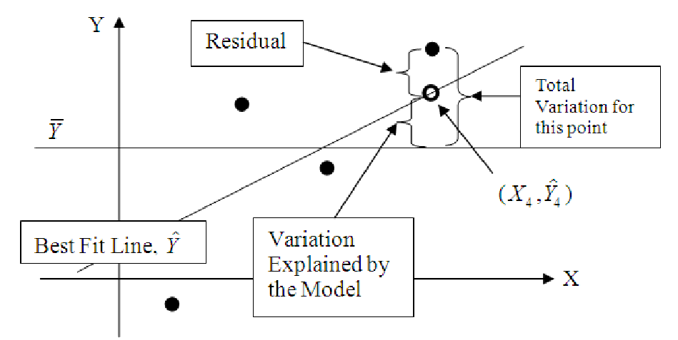
Residuals

This is the part that is left over after you use the explanatory variables to predict the y-variable. Each observation has a residual that is not explained by the model equation. Residuals are denoted by e_i and are computed by

e = y - ˆy i i i

Since these are computed from the y values, it should be clear that the residuals have the same units as the y, or response, variable.

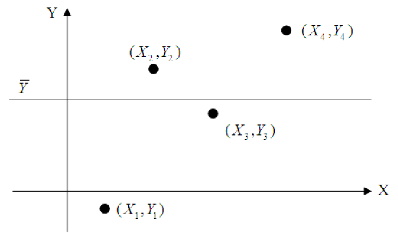
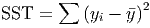
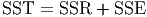
Total Variation (Total Sum of Squares, SST)

The total variation in a variable is the sum of the squares of the deviations from the mean. Thus, the total variation in y is

∑ 2 SST = (yi - y¯)

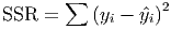
Unexplained variation (Sum of Squares of Residuals, SSR)

The variation in y that is unexplained is the sum of the squares of the residuals:

∑ SSR = (yi - ˆyi)2

Explained variation (Sum of Squares Explained, SSE)

The total variation in y is composed of two parts: the part that can be explained by the model, and the part that cannot be explained by the model. The amount of variation that is explained is

∑ ∑ SSE = Total Variation - Unexplained Variation = (yi - ¯y)2 - (yi - ˆyi)2

Regression Identity

One will note that the Total Variation is equal to the sum of the Unexplained Variation and the Explained Variation.

SST = SSR + SSE

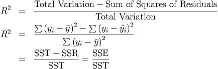
Coefficient of Determination (R²)

This is a measure of the ”goodness of fit” for a regression equation. It is also referred to as R-squared (R²) and for simple regression models it is the square of the correlation between the x- and y-variables. R² is really the percentage of the total variation in the y-variable that is explained by the x-variable. You can compute R² yourself with the formula

Total Variation - Sum of Squares of Residuals R2 = ---------------------------------------------- ∑ ∑ Total Variation 2 --(yi --¯y-)2----(yi---ˆyi)2- R = ∑ (y - y¯)2 i = SST---SSR--= SSE-- SST SST

R² is always a number between 0 and 1. The closer to 1 the number is, the more confident you can be that the data really does follow a linear pattern. For data that falls exactly on a straight line, the residuals are all zero, so you are left with R² = 1.

Degrees of Freedom for a linear model

The degrees of freedom for any calculation are the number of data points left over after you account for the fact that you are estimating certain quantities of the population based on the sample data. You start with one degree of freedom for each observation. Then you loose one for each population parameter you estimate. Thus, in the sample standard deviation, one degree of freedom is lost for estimating the mean. This leaves you with n - 1. For a linear model, we estimate the slope and y-intercept, so we loose two degrees of freedom, leaving n - 2.

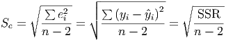
Standard Error of Estimate (S_e)

This is a measure of the accuracy of the model for making predictions. Essentially, it is the standard deviation of the residuals, except that there are two population parameters estimated in the model (the slope and y-intercept of the regression equation), so the number of degrees of freedom is n - 2, rather than the normal n - 1 for standard deviation.

∘ ------ ┌│ ------------ ∘ ------ ∑ e2i │∘ ∑ (yi - ˆyi)2 SSR Se = ------ = ------------= ------ n - 2 n - 2 n - 2

The standard error of estimate can be interpreted as a standard deviation. This means that roughly 68% of the predictions will fall within one S_e of the actual data, 95% within two, and 99.7% within three. And since the standard error is basically the standard deviation of the residuals, it has the same units as the residuals, whcih are the same as the units of the response variable, y.

Fitted values vs. Actual values

This is one of the most useful of the diagnostic graphs that most statistical packages produce when you perform regression. This graph plots the points (y_i,ŷ_i) . If the model is perfect (R² = 1) then you will have y₁ = ŷ₁, y₂ = ŷ₂, and so on, so that the graph will be a set of points on a perfectly straight line with a slope of 1 and a y-intercept of 0. The further the points on the fitted vs. actual graph are from a slope of 1, the worse the model is and the lower the value of R² for the model.

Residuals vs. Fitted values

This graph is also useful in determining the quality of the model. It is a scatterplot of the points (ŷ_i,e_i) = (ŷ_i,ŷ_i - y_i) and shows the errors (the residuals) in the model graphed against the predicted values. For a good model, this graph should show a random scattering of points that is normally distributed around zero. If you draw horizontal lines indicating one standard error from zero, two standard errors from zero and so forth, you should be able to get roughly 68% of the points in the first group, 95% in the first two groups, and so forth.

Figure 8.2: Sample initial data from which a regression line can be computed.

Figure 8.3: The various quantities involved in regression that are discussed above.

[next] [prev] [prev-tail] [front] [up]