Definitions and Formulas

Total change is a measure of the amount that a function changes from one data point to the other. Thus, if y is a function of the variable x we can find the value of y at two different x coordinates and then compute the total change in y. Note that the symbol ”delta” which looks like a triangle is the symbol for change:

Δy = f(x ) - f(x ) 2 1

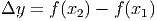
Notice that we always consider total change based on the assumption that the second x coordinate is larger than the first. In other words, we are looking at the change in y as x increases.

This is an idea similar to the slope of a straight line, but rate of change can be applied to non-linear models. Rate of change measures the steepness of a graph at a given point (more precisely, we are talking about instantaneous rate of change). The steeper the graph is, the larger the rate of change is. If the rate of change is negative at a point, the graph is decreasing at that point. If it is positive at a point, the graph is increasing at that point. If it is zero, the graph could be at a maximum or a minimum value, or could be at a saddle point. Measuring rate of change is what the first semester of calculus is really all about. For our purposes, we want to understand the rate of change as a number. It’s useful for telling us ”how much bang we get for each buck”. In other words, if we add more to the x variable (the bucks we spend) what does the rate of change say we get out (the bang). The rate of change of a function is closely related to the total change: usually we get at the rate of change through dividing the total change in Y by the total change in x. For linear functions, this number is the constant slope of the function. For nonlinear functions, the rate of change is level dependent.

In many cases, it is easier to interpret the percent change in a quantity than to interpret the total change or the rate of change of the quantity. Percent change in a quantity is the total change divided by the original amount. Thus, if we start at the point (x,f(x)) and move to the point (x + h,f(x + h)), the total change is f(x + h) - f(x), but the percent change in y is this divided by f(x):

y - y f(x + h) - f(x) -2----1 = ---------------- y1 f(x )

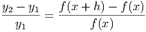
Notice that the percent change is a dimensionless number that represents a percent in decimal form. Thus, if the percent change of a model is 0.3 at a particular point, then this means that increasing x results in a 0.30 → 30% change in y at that point.

We’ve talked about this before, but it’s even more important now. Each number in a model (the constants, or parameters) will have some units associated with it. These units will help to interpret the meaning of the constant. So pay careful attention to the unit of measurement for each and every variable. Also note that the rate of change has units; these units are always the units of the response variable divided by the units of the explanatory variable.

Elasticity is an economic term for measuring the rate of change in a specific way. Elasticity is the actual rate of change divided by the current level. Thus, elasticity is really a measure of the percent change in the function, rather than a measure of the actual change (as the instantaneous rate of change is.) In fact, the elasticity of y with respect to x is the percentage change in y that results from a 1% increase in x.

Two functions, f and g, are inverses of each other if they satisfy the property that f(g(x)) = x and g(f(x)) = x. This means that if you do something to x (like apply f to it to produce the number f(x)) and then do its inverse to it, you get back to the number you started with, x. In this chapter, the two functions that are important, ln(x) and exp(x), are inverses of each other.

A way of using the idea of change and percent change to interpret the coefficients (parameters) in a nonlinear regression model. Note that this is not a standard term.

This is a way of interpreting the amount of change in a function. Specifically, marginal analysis is used to answer the question ”If the explanatory variable increases by one unit, by how much does the response variable change?”

You will need these properties in order to properly work with the regression output and convert it into a useable form. Sometimes you will apply these properties starting with the left side and converting it to the right side; other times you will have to go the other direction.

0 E1 b = 1 E2 brbs = br+s r s rs E3 (b ) = b E4 brs = br-s b

You will need these properties in order to properly work with the regression output and convert it into a useable form. Sometimes you will apply these properties starting with the left side and converting it to the right side; other times you will have to go the other direction.

r L1 ln(e ) = r L2 eln(a) = a L3 ln (a ) + ln(b) = ln(ab) ( ) L4 ln (a ) - ln(b) = ln a- b L5 r ⋅ ln (a) = ln(ar)

12.2.1 Definitions and Formulas