We have made extensive use of simple regression so far in this book. But how does simple regression work? How does the computer know how to compute the slope and y-intercept of the line that will minimize the total squared error in our approximation to the data? Wait a minute. That phrase ”minimize the squared error” sounds important. It sounds like we can use calculus to find the answer.
First, let’s do this with an example. Consider the following data points. We want to find the best fit (least-squares) regression line for these data.
| x | 1 | 2 | 3 | 4 | 5 |
| y | 5 | 7 | 8 | 9.5 | 12 |
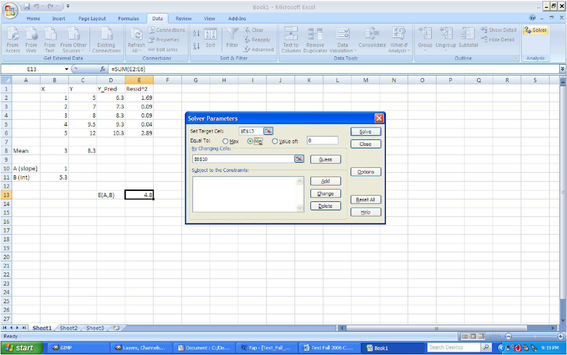
What we want to do is to minimize the total squared error between the data and the regression line. If the line has the regression equation y = A + Bx, fill in the rows of thespreadsheet (file C14 Regression.xls [.rda]) with the appropriate calculation for each data point. (For now, just guess a value of the slope and y-intercept. Place these values as parameters on the spreadsheet.) Now, add up all the squared errors to get the total error, E(A,B). This is a function of two variables, and we could treat it with calculus directly, but we’ll simplify everything slightly by noting that the regression line always passes through the point (,) which means that = A + B. Rearranging this, we get A = - B. Now, let’s put all this into the spreadsheet. You should have a sheet that looks a lot like the one below.
Now that we have the formulas entered, we can minimize the error function using the solver routine in Excel or the uniroot in R. Click on the cell containing the error value. Then click on ”Tools/ Solver” and enter the values as shown in the screen shot below. It should very quickly find the value of the slope (B) that minimizes the total squared error. Now run simple regression on the data (Y = response, X = explanatory) to see what the regression routine gives as the best values for the parameters.
If we do this in general, using calculus and algebra, we can find some interesting facts. The total error function will look like (remember, we have eliminated the A variable with the relationship above)
We can rearrange this last expression to be a little friendlier:
![∑n ∑n [ ]
E (B ) = [(yi - ¯y) - B (xi - ¯x)]2 = (yi - ¯y)2 - 2B (xi - ¯x)(yi - ¯y) + B2(xi - ¯x)2
i=1 i=1](Text_Fall_2014280x.png)
This can be rearranged a little to get an expression that really looks like a second degree polynomial in B (with ugly coefficients - but they’re just numbers!)

The derivative of this is just

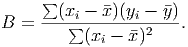
Setting this right hand side of this last expression equal to zero and solving for the parameter B we see that the error is minimized when