14.2.2 Worked Examples

Example 14.4. Using optimization to sketch polynomials
This example assumes that you have learned (from the last section) the following derivative rule:

Since a polynomial is just a sum of power functions, we can use this rule to determine the derivative of a polynomial: It’s just the sum of the derivatives of the individual power functions that make up the polynomial. Thus, the derivative of the polynomial f(x) = 3x⁴ - 5x³ + 2x- 7 is just f′(x) = 12x³ - 15x² + 2. (The derivative of 3x⁴ is 12x³. The derivative of -5x³ is -15x². The derivative of 2x is 2(1)x^1-1 = 2x⁰ = 2, and the derivative of a constant is zero.) We can use this to learn about the properties of polynomials and what they look like.

For example, suppose we have a general fifth degree polynomial. Thus, the function can be written (generally) as g(x) = a₅x⁵ + a ₄x⁴ + a ₃x³ + a ₂x² + a ₁x + a₀, where the a’s represent constants. What would the derivative of this function be? Well, we apply the power rule to each term and get: g′(x) = 5a₅x⁴ + 4a ₄x³ + 3a ₃x² + 2a ₂x + a₁. This is a fourth degree polynomial, as expected. How can this help us visualize the graph of g?

For starters, notice that if we try to find all the critical points of g we will have to solve the equation g′(x) = 0. This is a fourth degree polynomial equation and can have, at most, four solutions. Thus, there are at most four critical points in the graph of g. If we were to locate these critical points, we could begin to sketch the graph. Let’s take the specific polynomial h(x) = 6x⁵ + 15x⁴ - 130x³ - 210x² + 720x + 300. It’s derivative is h′(x) = 30x⁴ + 60x³ - 390x² - 420x + 720. To find the critical points, we set this derivative equal to zero and solve the equation. Since this equation can be factored as

we see that the derivative is zero at the points where x = 1,-2, 3,-4. There are four critical points. By plugging them into the function, we can find the y-coordinate of these points, and then graph them. Finally, we notice that since the leading term is a fifth degree power function with a positive coefficient, the function is increasing to the right. Since it is an odd-degree polynomial, it must do the opposite on the left, so it decreases to the left. In the end, we can sketch the graph quite accurately.

Example 14.5. Maximizing Profits with Derivatives
Suppose that the cost of producing q goods is

and we sell these goods for $7 apiece. How many of our product should we make (and sell) in order to maximize our profit?

The revenue function will be R(q) = 7q. This comes from the fact that revenue is simply the number of products sold times the selling price per product. The profit function (remember: profit = revenue - cost) will then be

The marginal profit is given by the derivative of the profit (which can be computed using the rules we have developed so far). We find that

We set this function equal to zero and do some algebra (anmely, the quadratic formula) to find that when q = 5.86 and q = 34.14 the profit function has a critical point. We can also get these results by entering the following data in our spreadsheet.

	A	B
1	q	1
2	P’(q)	=-0.03*B1+1.2*B1-6

In Excel, we can then use the goal seek procedure with the following information. ”Set Value” to B2, ”To value” 0, and ”By changing” B1. Note that this will only locate the first extreme point, q = 5.86. To be sure you do not miss the other points, it is good to first graph the function and visually locate some values that are close the extreme points. Then enter one of these values in cell B1. From the graph of P(q) we find that there is an extreme point near q = 30. If we enter 30 in cell B1 and then repeat the goal seek procedure described above (with B2, 0, and B1 in the ”Goal Seek” dialog box) the computer will locate the other extreme point. In R, we can use the uniroot to accomplish the same analysis.

Now, which of these two points is a maximum and which is a minimum? To answer this, we’ll apply the second derivative test. This is simple; we just find the second derivative of the profit function and evaluate its sign at each critical point. The second derivative of the profit function is just the derivative of the first derivative. So, we find

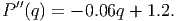
We then compute easily that P′′(5.86) = 0.8484, which is positive. This indicates that the point (q = 5.86,P = -16.57) is a local minimum - not a good place to be! At the other point we find that P′′(34.14) = -0.8484, so the point (q = 34.14,P = 96.57) is a local maximum for the profit function. That’s where we want our production and sales!

This tells us that if we sell our product at $7 each and incur a cost given by the function above then we can achieve a maximum profit of $96.57 dollars by making and selling 34.14 units of our product.

Example 14.6. Minimizing Average Cost
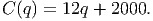
Suppose that we have a fixed cost of $2000 each month. This cost includes electricity, rent, and equipment. In addition, if it costs us $12 per good manufactured (including materials and labor), we have a total monthly cost of

Suppose that instead of minimizing the total cost, we now we want to minimize the average cost function. The average cost function, C(q), is basically the cost function divided by the quantity produced (i.e., average cost = total cost of making q goods divided by q.) Thus, the average cost function for this scenario is

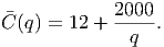
This is not a polynomial (the 1∕q term is really q⁽ - 1), which not a positive integer power) but we can use the sum rule and product rule to get its derivative:

Now, this function is not like our other examples: there is no minimum! We cannot solve the equation C′(q) = 0 because no value of q will solve this. However, we notice that as q increases, the derivative of the average cost decreases (the derivative is always negative.) This means that making more of our product will always reduce the average cost.

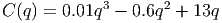
If, instead, we had a slightly more realistic cost function (taking secondary costs into effect) like

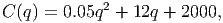
then we can optimize the function. Following the same steps as before, we get the average cost function as

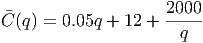
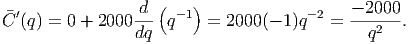
and we find its derivative as

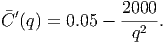
Setting this derivative to zero, we get

Thus, to minimize the average cost of producing the goods, we should make 200 goods. This is especially useful, since the cost function itself is only minimized for a negative number of goods! (Try it. You should get the derivative of the cost function as C′(q) = 0.1q + 12 which is minimized at q = -12∕0.1 = -120 goods.)