
Example 15.4. Compound interest formulas
Suppose we were to invest an amount of principal, P, in an account that earns an interest rate r
each year (this is the APR, or Annual Percentage Rate). This means that at the end of the first
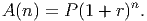
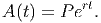
year, you will earn rP additional money. Thus, after one year, your account, A, has the
value
If you were to leave the money in the account for a second year, you would earn interest not only on the principal, but also on the interest you earned the first year:

What if you let the money earn interest for a third year? You would have a total of

With a little work, we can show that, in general, after n years at an APR of r your principal P will earn a total of
Now, suppose that our interest is not computed annually, but is computer every month, based on the APR. This means that the actual monthly interest rate is r∕12 and that in a single year we have 12 compounding periods. Similar logic to the previous case will tell us that after t years of compounding the interest monthly at this rate we will have
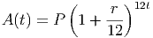
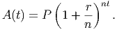
dollars in the account. Similarly, if we let the money be compounded n times each year, we will have an interest rate of r∕n each period and a total of nt compounding periods after t years. This gives us an amount of
This is, obviously, an exponential function, but with a base of (1 + r∕n) rather than the natural base of e. However, they are related. Consider what happens if we invest $1 at 100% APR for one year under different compounding periods, as shown in the table below.
| Schedule | Number of Periods | Total Amount |
| Annual | 1 | 2 |
| Monthly | 12 | 2.61303529 |
| Weekly | 52 | 2.692596954 |
| Daily | 365 | 2.714567482 |
| Hourly | 8760 | 2.718126692 |
| Each minute | 525600 | 2.718279243 |
| Each second | 31536000 | 2.718281781 |
| Every tenth of a second | 315360000 | 2.71828187 |
| Every hundredth of a second | 3153600000 | 2.718281661 |
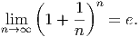
Notice that the amount of money does continue to grow, but not at the same rate. In fact, it seems that the amount of money we are earning is approaching a fixed amount. Mathematically, it is has been proven that this is the case and that the number this approaches is the number e:
The number e is the amount of money earned in an account after investing $1 for one year at 100% interest, compounded continuously.
Mathematicians write this fact using the limit notation:
We can now use this fact to generate a formula for continuously compounded interest. First, we introduce a new variable m so that n = r ⋅ m. Then we have an equivalent expression for the interest given by
![( r)n ( 1)mrt [ ( 1)m ]rt rt
nl→im∞ 1 + n- = lmi→m∞ 1 + m- = lmi→m∞ 1 + m- = e .](Text_Fall_2014320x.png)
Thus, our formula for the amount in an account with n compounding periods changes to the following formula if we compound it continuously:
Example 15.5. Derivatives of exponential functions
Now that we know about the derivatives of logarithmic functions, we can easily use the idea of a
logarithmic derivative to determine the derivative of an exponential function. One of the most
common exponential functions to occur in the business world relates to the future value
of an investment. To get to this, though, we’ll need to develop the idea of compound
interest.
So, although it took us a little while to get there, and we skipped a few steps, we see that the exponential function is closely tied to the idea of compound interest. We can now ask the following. Suppose you have invested a fixed amount of money P at a fixed rate of interest r. How quickly (in time) is your money growing in value?
The question ”how quickly” immediately reminds us of the idea of rates of change, so we know we are really talking about the derivative of the amount of money in the account. So, what is the derivative of the amount? We’ll use our knowledge of logarithmic derivatives to help. We really want to know the derivative of A(t), but we don’t know the derivative of an exponential. However, the exponential function and the logarithmic function are inverses of each other, so the formula for the amount can be rewritten as

where we have used the rules for manipulating logarithms and the fact that ln(e) = 1. Now, we can take the derivative of each side of this equation, using the chain rule:
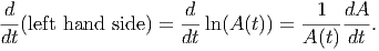
Now, the derivative of the right hand side is easy, since it’s really a linear function (note that ln(P) is a constant; it doesn’t depend on the variable t with respect to which we are taking the derivative):

We can now put all this together, since we have done the same thing to both sides of the equation (namely, take the derivative with respect to t), so they are still equal to each other.
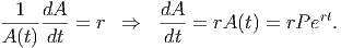
So, the true rate of increase of your account value is an amount of r * exp(rt) dollars per year. If you let it sit for t = 10 years at a rate of 2.5% your money will be increasing at a rate of A′(10) = 0.025 ⋅ P ⋅ exp(0.025 * 10) = 0.025 ⋅ P ⋅ exp(0.25) = 0.032P dollars per year. If you had invested $1000 initially, this would come to a growth rate of about $32/year.
Example 15.6. Derivative of an exponential function
Find the relative rate of change of the function g(r,t,P) = Pert with respect to the
variable r. The relative rate of change is just the rate of change divided by the function
itself, so we have the relative rate of change as (1∕g)⋅ (derivative of g with respect to
r).
  = =   (Pert) (Pert) |
| Definition of relative rate of change, using partial derivative notation since there are several variables in the function |
=  ⋅ P ⋅ ⋅ P ⋅ (rt) (rt) |
| Derivative of a constant times a function |
=  ⋅ P ⋅ ert ⋅ r ⋅ P ⋅ ert ⋅ r |
| Derivative of an exponential AND chain rule |
=  ⋅ r ⋅ g ⋅ r ⋅ g |
| Derivative of a linear function |
| = r |
| Simplification |
This means that the relative rate of change of the formula for continuously compounded interest is just equal to the interest rate itself. To understand what this means, think about the units of the rate of change with respect to r: units of dollars divided by units of interest. When we divide this by the amount (dollars) we get the relative rate of change, which is measured in 1/(interest rate). This is a relative amount, so it is like a percentage. Thus, each actual 1% increase in the interest rate (from 1% to 2% or from 5.25% to 6.25%) will increase the value of our account for a fixed amount of principal invested for a fixed period of time by r %.
Example 15.7. Application of Marginal Analysis to Business Decisions
The analysis team at Koduck has determined the following information about your current
production level:
Marginal cost (MC) = $2.25/unit
Marginal Revenue (MR) = -$1.15/unit
What does this mean for Koduck?
For starters, we note that a negative value for marginal revenue means that if you increase production by 1 unit, your overall revenue (price * number sold) will actually drop. (This could be because you have already flooded the market; after all, how many pictures of water fowl can you sell in a given city?) The fact that the marginal cost is positive means that it will cost you more to make one more unit of product. Thus, it seems that increasing current production levels would not be wise: The total cost would rise and the revenue would drop, leading to lower profits. No one wants that. In fact, we should probably decrease production in order to increase profits! If we decrease production by 5 units, say, then we can expect the revenue to increase:
Change in Revenue = MR*change in production = (-$1.15/unit)*(-5 units) = $5.75.
At the same time, this would result in a decrease in cost:
Change in Cost = MC*change in production = ($2.25/unit)*(-5 units) = -$11.25.
This results in a total change in the profit of $17! It is a fact (which we will explore later) that the maximum possible profit (= revenue - cost) must happen when the marginal cost and the marginal revenue are equal. Since we can increase profits by lowering production, we must be producing more units than necessary to achieve the maximum profit.