3.1.1 Definitions and Formulas

Model

A model is a number or formula that represents a set of data; it is not the data itself, but is meant to capture certain important features of the data that would otherwise not be recognizable. Models can be descriptive (used to describe a particular situation or set of data), predictive (used to help understand the likely future outcomes of a situation), or interpretive (designed to help one understand how the current situation came about or where the data came from), and can take the form of numbers, graphs, pictures, equations or descriptions.

Empirical Model

An empirical model is based only on data and is used to predict, not explain, a system. An empirical model usually consists of a function that captures the trend of the data

Statistic

Any number used to represent some aspect of many observations of a single variable or that relates several variables together. For example, the mean is one way to describe a list of numbers; it reduces the entire list to a single statistic representing the typical data point.

Central tendency

A statistic that is intended to provide a measure of what a ”typical” data point is for a single variable. The most common measure of central tendency is the arithmetic average, or mean. Others include the median, mode and geometric average.

Mean

An average computed by adding all the observations of a variable together and then dividing by the number of observations. This is more properly called the arithmetic mean. This is the most commonly used average, and it is the most robust average (it will change the least under repeated sampling of the population). In symbols, the mean of the data x₁,x₂,x₃,…,x_n is

Sigma, Σ

This symbol provides a compact way to represent adding a large number of items together if they follow a pattern. For example, the formula ∑ _i=1⁵(i + 2) means that we are adding together five objects that look like i + 2, that is, each object is a number, i, plus 2. So, the first term in the sum starts at the smallest value of i (in this case, 1) and increments up for each term. So, the nice compact formula really represents a much larger addition problem:

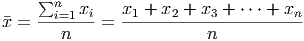
The sigma notation (the symbol is the uppoercase Greek letter S, for ”sum”) provides a much cleaner way to write the formula. After, all, if we had to add from i = 1 to i = 10, 000, writing each term out by hand would be tedious and rather pointless.

Deviation

The deviation of a data point is its signed distance from the mean. To calculate this for data point x_i simply subtract the mean from the data point: x_i -x . This deviation will be positive if the observation is larger than the mean and negative if the deviation is smaller than the mean.

Total Variation (SSD)

This is the sum of the squares of all the deviations of all the observations in the data. In symbols, this is

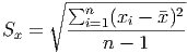
The total variation is always positive (since you are adding a bunch of squares of numbers) or zero (if each observation is equal to the mean).

Sample Standard Deviation

This is a sort of average deviation for all the observations in the data. The sample standard deviation for a set of data labeled x is denoted by the symbol S_x. To compute this, we take the total variation in the data (see above), divide by the number of degrees of freedom (usually n - 1) and then convert back into the right units by taking the square root:

Degrees of Freedom (DOF)

This is related to several key ideas: the number of observations in your data and whether the data is from a population or from a sample. If the data is from a population, then the number of degrees of freedom is the same as the number of observations. However, if you are taking data from a sample and calculating quantities (such as the mean) that describe the population, then you lose a degree of freedom for each calculation you are inferring about the population. For example, to compute the standard deviation of a sample, you must calculate the (inferred) mean of the population. This costs you one degree of freedom, taking you from n to n - 1.