
Example 3.1. Computing a mean
For this example, we want to compute the mean of a set of test scores:
55, 60, 67, 70, 78, 81, 84, 88, 90, 95, 99
The mean of the data is given by adding the observations and dividing by the number of observations, n = 11. Thus, the mean of this data2 is
Thus, we would say that a typical student received a score of about 79 on this test.
Example 3.2. Deviations and average deviations
Computing the deviation of a data point from the mean is simple. We just subtract the mean from
the data point. The result is a signed number (it could be positive or negative) that tells us how
far the data point is from the mean. So in the data for burgers at Beef n’ Buns, we can
compute the deviation of each burger’s fat content from the mean fat content of 34.7
g.
| Item | TotalFat | Deviation |
| Super Burger | 39 | 4.3 |
| Super Burger w/ cheese | 47 | 12.3 |
| Double Super Burger | 57 | 22.3 |
| Double Super Burger w/ Cheese | 65 | 30.3 |
| Hamburger | 14 | -20.7 |
| Cheeseburger | 18 | -16.7 |
| Double Hamburger | 26 | -8.7 |
| Double Cheeseburger | 34 | -0.7 |
| Double Cheeseburger w/ Bacon | 37 | 2.3 |
| Veggie Burger | 10 | -24.7 |
From this, it is clear that the veggie burger has much less fat than the typical Beef n’ Buns burger, while the Double Super Burger with Cheese contains considerably more fat than the average sandwich. Also notice that none of the burgers is actually right at the average fat content of 34.7 g; the Double Cheeseburger is close, but a little low. Given this, if we randomly chose a burger to eat, what would we expect its fat content to be? This is really just another way to ask what the average deviation of the fat content is.
Well, this is just an average of the deviations, right? So we can add up the deviations and divide by the number of burgers. Unfortunately, we find that the sum of the deviations is zero, giving an average deviation of zero. But how can this be? Not only do none of the burgers have exactly the mean fat content, but many of them are quite far away from the mean. (Just in case you think we have rigged this example, try it with the protein content of the burgers. Then try it with any list of numbers you want to use - your favorite football team’s points per game, for example.)
In fact, the sum of the deviations from the mean is zero, for any set of data points. We can use some algebra to decide whether this conjecture is really true.
Old Data = xi
Old Mean =
New Data = xi -
Now simply add all these data points up and compute the mean of the new (shifted) data:

Notice that this calculation works in general. We did not need to have a specific set of data, or a specific mean, or a specific number of data points. By using algebra we can show that the mean of the deviations of any set of data is zero (and thus, the sum of the deviations is zero). This example shows both the power and beauty of mathematics. Rather than work hundreds of examples and rather than calculate each sum of deviations separately, we now have a powerful understanding of what is beneath the actual data.
Why does this happen? Another way to calculate the mean is to ”take from the tall and give to the small”. The amount you take from the tall (large data values) is equal to the deviation for that stack. The amount that the small needs is the deviation for that stack, which is a negative number. So the mean is gotten by making all the deviations zero. Thus, the reason for the sum of the deviations equaling zero is related to the fact that some deviations are positive and others are negative. Adding the positive and negative numbers cancels out the deviations completely.
What does this result mean, in practical terms? It means that since the sum of the deviations is always zero, we cannot use the deviations themselves to compute an ”average distance from the mean”. We must construct a new tool to measure the typical distance of an observation from the mean of the data.
Example 3.3. The Standard Deviation Formula: What it all means
The last example showed that the sum of the deviations is always zero because there is always the
same total amount of positive deviation (above the mean) as there is negative deviation (below
the mean). What we need is a way to turn all the deviations positive; after all, we are
really interested in the average distance of the observations from the mean, not in which
direction the observation falls. What ways can we take positive and negative numbers
and make them all positive? If you’re like most people, you can think of at least two
ways:
For technical reasons, mathematicians prefer the second method, squaring all the deviations. If we then add up the squared deviations, we get the total variation of the data:
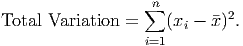
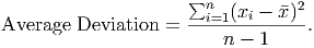
This number by itself is not very useful. First of all, no matter what the units of the original data were, the total variation is never in those units; it’s always measured in the square of those units. Thus, if the original data were measured in dollars, the total variation would be in square-dollars, whatever those are. Second, the total variation is the sum of a bunch of squared numbers. If a number bigger than 1 is squared, the result is much larger than the original number. Thus, the total variation is often a huge number. Third, this is a total amount, not an average amount. This leads us to the next step: divide by the number of degrees of freedom to compute an average variation:
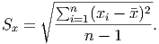
This number still suffers from the problems of being in the wrong units and being huge. But this is relatively easy to fix. We got the numbers larger and into the wrong units by squaring them. What’s the opposite of squaring a number? Taking the square root! (The squaring function and the square root function are inverse functions.) This one simple solution will make the numbers smaller and put them into the proper units. We are then left with the sample standard deviation3 :
So you can see that although the formula for the standard deviation looks complicated, every piece of it is in the formula for a specific reason. For the data listed in example 2, we can determine the standard deviation. (Remember, the mean is 34.7.)
| Item | TotalFat | Deviation | Squared Deviation |
| xi | xi - | (xi -)2 | |
| Super Burger | 39 | 4.3 | 18.49 |
| Super Burger w/ cheese | 47 | 12.3 | 151.29 |
| Double Super Burger | 57 | 22.3 | 497.29 |
| Double Super Burger w/ Cheese | 65 | 30.3 | 918.09 |
| Hamburger | 14 | -20.7 | 428.49 |
| Cheeseburger | 18 | -16.7 | 278.89 |
| Double Hamburger | 26 | -8.7 | 75.69 |
| Double Cheeseburger | 34 | -0.7 | 0.49 |
| Double Cheeseburger w/ Bacon | 37 | 2.3 | 5.29 |
| Veggie Burger | 10 | -24.7 | 610.09 |
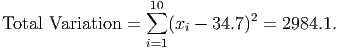

This says that, on average, most data points (approximately 68% of the data points) are within 18.21 units above and 18.21 units below the mean. This would give a range of - Sx = 34.7 - 18.21 = 16.49 up to + Sx = 52.91 for most of the data. By counting the data points, we see that 6 out of the 10 data points (60%) fall inside this range. Going out to two standard deviations above and below the mean should give us 95% of the data. The lower end of that range would be - 2(Sx) = 34.7 - 2(18.21) = -1.72 and the upper end would be + 2(Sx) = 71.12. We see that the data has all 10 points (100%) within this range.
In general, if the data is normally distributed we expect the following empirical rules to be true:
We’ll learn more about checking and applying this rule in the How To Guide. For now, it’s enough to know it exists. It is also the basis for a popular management system known as ”Six Sigma” or 6σ. This refers to the use of the symbol σ (a lowercase Greek ”s”) for the standard deviation. One of the goals of the Six Sigma method is to minimize the amount of production (or whatever you are involved in that can be measured) that falls outside of three standard deviations above and below the mean. At most 0.3% of all data should fall that far away.
Example 3.4. Using Means and Standard Deviations to Compare Sales Performances
The data below shows the total monthly sales for each branch of Cool Toys for Tots in two
different regions of the country, the north-east region and the north-central region. (See file C03
Tots.xls [.rda].) Which of these two regions is performing better?
| Sales NE | Sales NC |
| $95,643.20 | $668,694.31 |
| $80,000.00 | $515,539.13 |
| $543,779.27 | $313,879.39 |
| $499,883.07 | $345,156.13 |
| $173,461.46 | $245,182.96 |
| $581,738.16 | $273,000.00 |
| $189,368.10 | $135,000.00 |
| $485,344.87 | $222,973.44 |
| $122,256.49 | $161,632.85 |
| $370,026.87 | $373,742.75 |
| $140,251.25 | $171,235.07 |
| $314,737.79 | $215,000.00 |
| $134,896.35 | $276,659.53 |
| $438,995.30 | $302,689.11 |
| $211,211.90 | $244,067.77 |
| $818,405.93 | $193,000.00 |
| $141,903.82 | |
| $393,047.98 | |
| $507,595.76 | |
One way to answer this question is to compare the mean sales in each region. We find that the northeast region has mean sales of $325,000, and the north-central region has mean sales of $300,000.
Based on this information, we might conclude that the northeast region is doing better. But we must consider whether the mean is a good way to model this data. As a clue, when looking at the northeast region, we notice some of the lowest performing stores in the sample! And notice that there is one store in the north-east region with sales of $818,405.93. This is much higher than the sales for the other stores in either region. This single high value is pulling the mean for the north-east region up, even though the stores in the north-central region are typically doing better, as evidenced by the fact that many of them (almost half) are well above the north-central region’s mean. In the northeast, however, the stores performing below the mean are typically far below the mean.
This sensitivity to high or low scores is one of the drawbacks of the mean. This is why the Olympics (and many other sports bodies) drop the high and low scores for a competitor before computing the mean. In later chapters, you’ll learn what data points like this are called and gain a powerful graphic tool for determining which data points are likely to have too much influence on the mean.
We already know that the mean of the NE region sales is $325,000 and the mean of the NC region is $300,000. What about the standard deviations for each region?
| Sales NE | Sales NC | |
| Mean | $325,000.00 | $300,000.00 |
| Standard Deviation | $217,096.62 | $141,771.13 |
Now we have some useful information. The NE region has a much larger standard deviation than the NC region. In the NC region, though, this smaller standard deviation indicates a much narrower spread of the data. This means that the stores will perform more similarly to each other, indicating more consistency and more stable, dependable sales results in the long run. The stores in the NE region are, on average, more spread out than those in the NC region. We are likely to have very high and very low sales in this region. Notice the last store on the list for the NE region. It had sales of $818,405.93, which is very high compared to the other stores. This store is a potential outlier (a data point so atypical that we should not consider it.) What happens if we remove it from the data?
| Sales NE (without outlier) | Sales NE (with outlier) | |
| Mean | $292,106.27 | $325,000.00 |
| Standard Deviation | $178,742.58 | $217,096.62 |
Notice the dramatic change in the results! Although the NE region (minus the outlier) is still slightly more spread out than the NC region, it is nowhere near as spread out as it was. Also, the mean for the NE region without the outlier is now slightly below the mean of the NC region. This shows you how important a single observation of the data can be. If you have outliers in the data, it is a good idea to report the statistics with and without the outliers. In this case, the $292,106.27 value is more representative of the bulk of the stores in the NE region than the $325,000 value, which was exaggerated by the outlier. Also, without the outlier, the stores in the NE region have more similar sales results, indicated by the smaller standard deviation.