In the last group of exercises, we discovered that the straight line solutions (if any) of a system of linear, homogeneous ODEs were easy to find: Assume that y = kx and plug that into the phase plane equation (dy/dx = g/f). Solve this for k to find the slopes of the straight line solutions. Then, one can use these special solutions in the phase plane to find the component solutions x(t) and y(t) by plugging y=kx into each of the equations of the system.
In general, though, this is not an efficient method for finding the special solutions and the component solutions. Instead, we'll look at the matrix describing the system. If we write this matrix as A (defined below) then there is a "characteristic polynomial" for A that will help us find everything about the system.
Each matrix A has two numbers associated with it. One is called the trace of A and the other is called the determinant of A. The trace of A is denoted as Tr(A) and the determinant is det(A). For a 2 X 2 matrix with entries as shown above, the trace and determinant are simple.
The trace of a matrix is the sum of the entries along the main diagonal (upper left to lower right corner). This definition holds for any square matrix. Thus, for our matrix above, the trace is simply (a11 + a22).
The determinant is more complicated to define for a general matrix, but for a 2 X 2 matrix, we multiply the entries on the main diagonal and subtract the product of the entries along the other diagonal (upper right to lower left). Thus, det(A) = a11a22 - a12a21.
Technically, the characteristic polynomial is computed by subtracting an unknown quantity (usually lambda) from each entry on the main diagonal. The determinant of this matrix is the characteristic polynomial of the matrix. However, in all cases, it turns out that the characteristics polynomial is simply
![]()
Setting this equal to zero and solving produces the eigenvalues of the matrix. Each eigenvalue is associated with an eigenvector. As it turns out, these eignevectors are the straight line solutions in the phase plane!
You'll also notice that the characteristic polynomial is a quadratic polynomial in lambda. This means that we could find that there are
As it turns out, there is another important case: when one or both of the eigenvalues is zero. Each of these different cases will produce different types of equilibrium points at the origin for our system.
Using the eigenvalues, we can determine the basic behavior of solutions near and equilibrium point. A lot of work has gone into this, and it is all summarized in the diagram below, taken from Selwin Hollis's text Differential Equations with Boundary Value Problems.
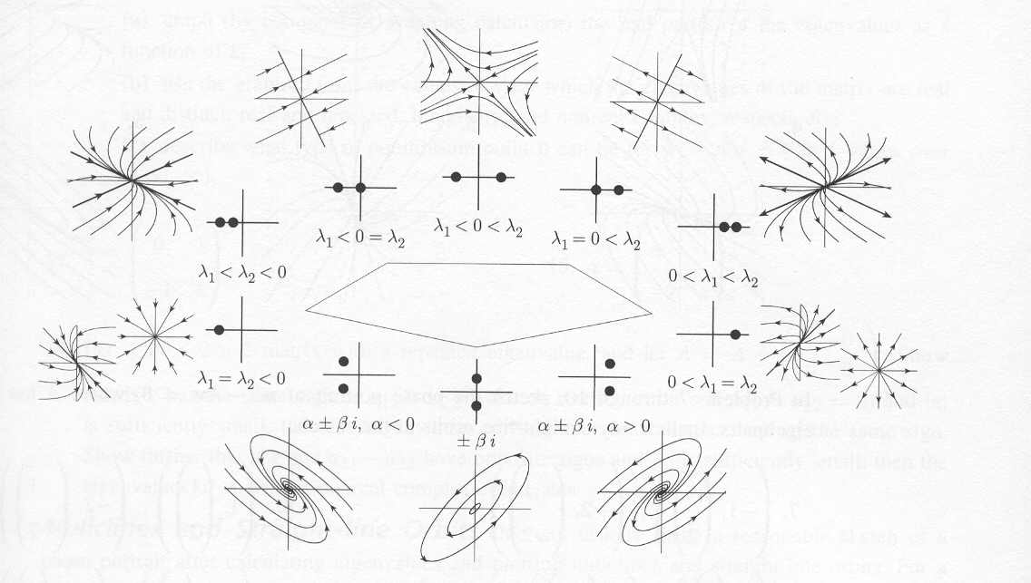
In the diagram, you see there are two graphs for each equilibrium point: the outer graph shows a phase plot of the point, while the inner graph plots the eigenvalues in the complex plane (the vertical axis is the imaginary component of the eigenvalue and the horizontal axis is the real part). Each diagram also includes a symbolic description of the eigenvalues.
For example, if you find that the eigenvalues are both real, with one positive and one negative, then the equilibrium point must be like the one in the top center of the diagram: a hyperbolic equilibrium point. If the eigenvalues are complex, with a negative real part, then the equilibrium point is shown on the bottom row, just left of center.
The pentagon in the center of the diagram is there to separate the equilibrium points into two cases:
MAPLE has a package that can be loaded to analyze the matrix of a system of ODEs and then you can use this to determine the complete solution to the system. The commands are given below, in red. The information to the right of the command is a comment to explain what the command is doing. Don not enter the information on the right into Maple.
| > with(linalg): | load the LINear ALGebra package for the definition and manipulation of matrices |
| > A := matrix(2,2, [[0, 1], [-2, -3]]); | define A as a 2 x 2 matrix (rows, columns) with the first row as 0 1 and the second row as -2 -3. |
| > eigenvalues(A); | returns the eigenvalues of A |
| > eigenvectors(A); | returns a lot of information: the eigenvalues, the
multiplicity of each eigenvalue (the number of times it occurs), and the
eigenvector associated with each eigenvalue. This is in the format: [first e-value, multiplicity, {[first e-vector]}], [second e-value, multiplicity, {[second e-vector]}],... |
QUESTION 11. Use MAPLE to classify each of the following systems of ODEs. Find the eigenvalues, sketch the eigenvectors as lines in the phase plane, and then sketch solutions to show their behavior. Use the classification diagram above to help you.
| A. |  |
B. |  |
| C. |  |
D. |  |
| Back to previous screen |
Next screen |
Written and posted by Dr. Kris H. Green, March 24, 2004