We have spent some time considering problems that involve data. Usually the data contains observations of several variables, but so far, we have concentrated on understanding each variable separately with statistical methods (like the mean and quartiles) or graphical methods (like boxplots and histograms). Now we are moving into the heart of this book: analyzing the ways in which one or more variables may influence another variable. We are going to start slowly, by analyzing relationships between two variables. We will quickly see the power of graphs for showing the relationships, but we will also see the limitations of such approaches. We’ll build on the graphs by developing some numerical methods of determining relationships and their strengths.
But the real heart of this book is in the application of mathematics to construct a model of the data. This means that we must eventually develop equations that embody the relationships between the variables. We will start with some data and then try to build an algebraic description of the data. Once we have this description, we can begin to make predictions, test the predictions, and use these tests to refine the model. After we have developed a reasonable model of the data, this model will enable us to understand the relationships between the variables much better than a list of numbers or even a graph.
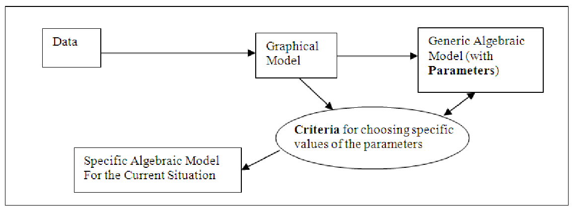
Schematically, the method we will use to develop these equations looks something like this:
You will notice two new terms in the above diagram: parameters and criteria. In order to gain an understanding of these terms, we are going to explore many examples. As you will discover later, most of the types of algebraic models are pretty well understood. They always have the same sort of equation to represent them, but may have different numbers in the equations. These constants can be changed in order to make the general model fit the specific data you are dealing with. In order to choose good values of these parameters, though, we’ll need to define criteria that let us select the best values. In the present unit, all our models will be from one category that you have probably encountered before: linear equations. These are the easiest to understand and to interpret, so they are often used as a starting point to analyzing data.
When we use mathematics to help us understand a problem situation, we are often interested in finding how one variable quantity relates to the value of another variable quantity. In particular, we would like to be able to identify which one depends on the other for its value and then, hopefully, to be able to figure out precisely what that relationship is. The variable quantity that depends for its value on the other is called the dependent variable and the other variable quantity, the one upon which the dependent variable depends, is called the independent variable.
We often call the dependent variable the output variable (or simply output) and the independent variable the input variable (or input) because we are trying to get a precise description of some kind of causal or linking mechanism connecting the two. So we think of inputting various numbers into the mechanism and then watch the corresponding outputs. If we have correctly, or at least adequately, described the connecting link between the input and the output variables, the resulting outputs should match what we actually find in our problem situation. We can then use this input/output linkage to predict what will happen in circumstances for which we have no actual data.
Not all relationships between variables, however, are useful, particularly when they lead to ambiguous results; that is, more than one output for a given input. When this happens, we don’t know which output to associate with the given input since there is more than one possibility. For example, think of the price you pay for an airline ticket and the distance you fly. It would seem reasonable that the cost should depend on the distance you fly. You probably know from experience, however, that you could pay very different prices for a flight of 400 miles from your point of origin, depending on, say, the day of the week or a special discount. An input of 400 mi. for the independent variable, distance, could produce two output prices (or more), say $200 and $250, for the dependent variable, cost. Our relationship between the input and output produces ambiguous results since we cannot predict what the output price of the 400-mile ticket will be2 .
A relationship between variables in which a single input3 produces only one output is called a function. Functions can be represented, as we have seen, as tables, graphs, or rules (equations). Here are some connections among the three ways of representing functions:
Before we can begin any of the above steps, however, we have to identify what we think the independent and dependent variables might be in a given problem situation. At this preliminary stage of our analysis, a graph of the possible relationship between the two variables is an extremely simple and effective way to test whether we have identified the independent and dependent variables correctly, as well as to form a basic notion of how the independent variable relates to the dependent variable.