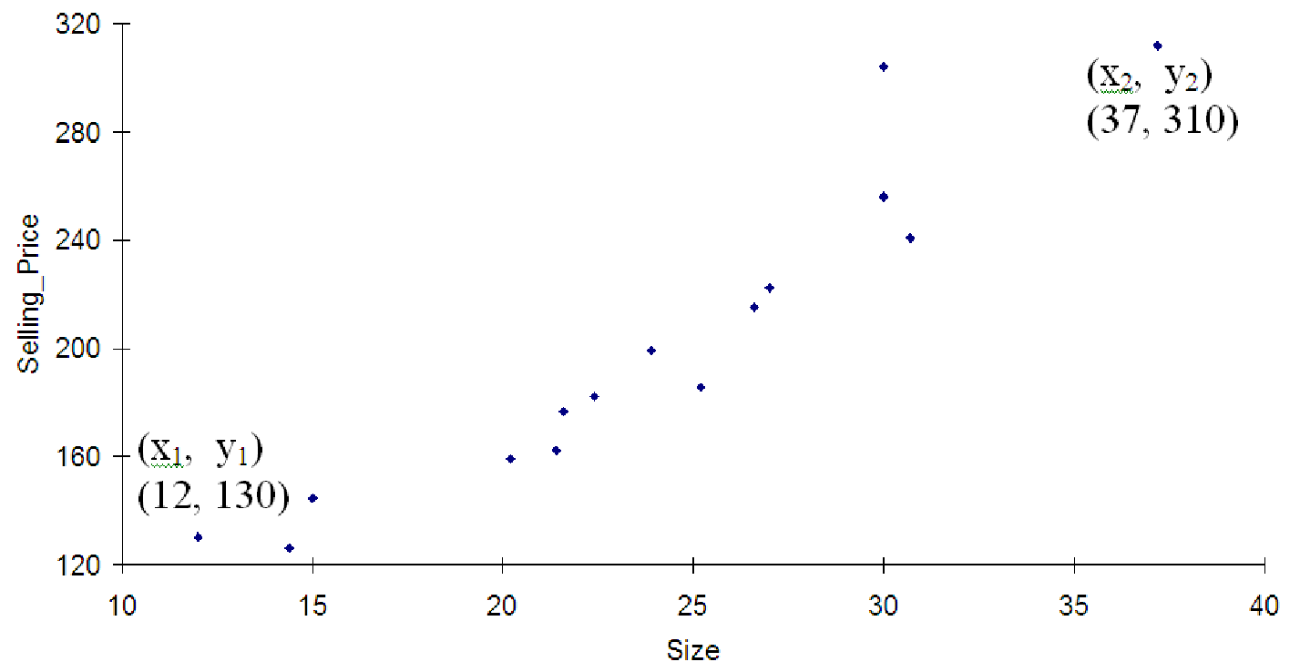
Figure 7.12: Plot of home selling prices (dollars) versus home size (square feet).
The easiest relationship between two variables to model is a linear relationship. Straight lines are easy to picture, they have simple equations, and each part of a straight line equation can be easily interpreted into real-world terms. Consider the data shown in figure 7.12. The independent variable is the size of a home in hundreds of square feet and the dependent variable is the price of the home in thousands of dollars. The data were taken from a sample of fifteen homes in a single neighborhood that all sold within one year. The graph clearly indicates a strong linear relationship between the two variables: larger homes tend to have higher prices.
We can easily draw a straight line through this data that does a reasonable job representing the data. But what do we really mean by ”representing the data”? Clearly we cannot draw a single straight line which passes through all of the data points. How then do we decide what the best line is? Each line is characterized by two numbers, slope and y-intercept. By carefully choosing these numbers we can make the line fit the data better. But how? Slope is basically the tilt of the line: larger values make the line more tilted, positive values tilt up, and negative values tilt down. The line for this data must have a positive slope. Furthermore, since the two extreme data points are about (37, 310) and (12, 130) we see that an increase in size of 37 - 12 = 25 hundred square feet results in a price increase of 310 - 130 = 180 thousand dollars. Thus, the slope of the line is approximately 180/25 = 7.2 thousand dollars per hundred square feet of size.
Now that we have an estimate of the slope for this line, we can compute the y-intercept. Since the equation of the line is y = A + Bx where B is the slope we just found (7.2), and since the line must pass through one of the points we used, we can plug all the known information into the equation and use algebra to find the value of A that makes the line with that slope pass through that point. So, we have 310 = A + 7.2 * 37. We want to solve for the unknown A. We find that A = 43.6. Thus, we might estimate the line as y = 43.6 + 7.2x.
In this section, we will explore the equations of straight lines and use them to model relationships between two variables. We will also see how these equations can be used to make predictions about data that is not part of the data set. This involves specifying a value of the independent variable and calculating the dependent variable from the equation. We will also see how to determine values of the independent variable that give rise to specified values of the dependent variable. This is usually referred to as ”solving an equation.”