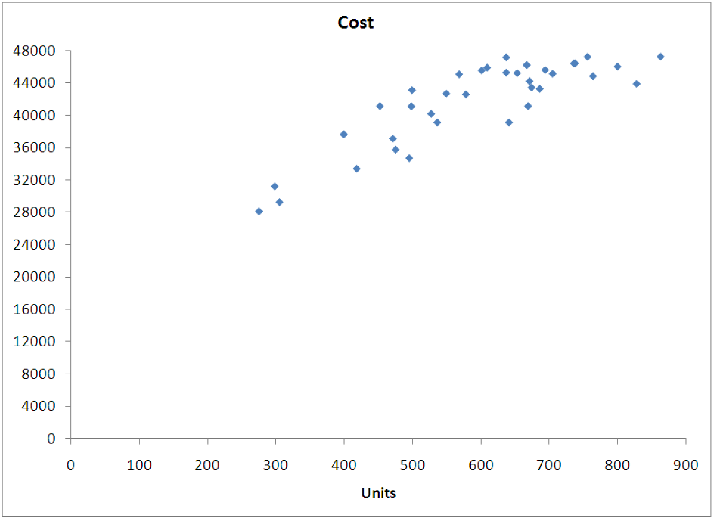
Figure 13.1: Electricity cost versus units used illustrating a nonlinear (possibly parabolic)
relationship.
In a previous chapter, we discussed building models using interaction terms. However, we only dealt with two of the three types of interaction terms: the interaction of two categorical variables and the interaction of categorical variable with a numerical variable. In this section, we will talk about what happens when you allow two numerical variables to interact, and what happens when you interact a variable with itself.
The second case is actually slightly easier to understand. Interacting a variable with itself produces a new variable in which each observation is the square of one of the observations of the base variable. Thus, a model built from a variable interacted with itself is a nonlinear model, specifically a square or quadratic model. This gives us another way to think about creating simple nonlinear models. Consider the data shown in the graph below, which has indication of being a parabola. The independent variable is Units (of electricity) and the dependent variable is Cost.
We can easily produce a quadratic model, and we find it has the equation
Cost = 5792.80 + 98.35 ⋅ Units - 0.06*Units ⋅ Units.
This model is clearly a parabola. It opens downward (as the graph shows) since the coefficient of the variable ”Units ⋅ Units” is negative. (Of course, we don’t expect there to be a discount for using too much electricity, so a quadratic model is perhaps not the most appropriate here, but you get the picture.)
The other situation - interacting two different numerical variables - is much harder to visualize, since we are dealing with at least three dimensions (one for each of the base variables plus one for the dependent variable). In the next section, you will work on interpreting such models and getting some sort of picture of what they might look like. For now, though, we concentrate on generating models of these two types, which are both quadratic models.