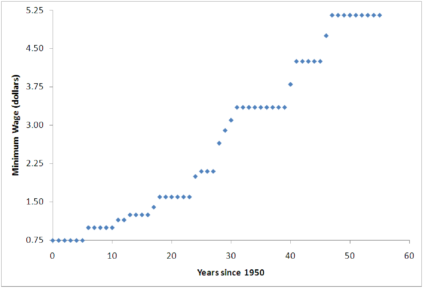
Figure 13.2: U.S. minimum wage versus years since 1950.
Example 13.1. Models built with one variable and self-interaction
Consider data on the Federal minimum wage, shown in C13 MinWage.xls [.rda]. This data shows
the minimum wage (in dollars) at the end of each calendar year since 1950. Suppose we would like
to build a model for this data in order to make projections about future labor costs for running a
small company. Thus, we seek to explain the minimum wage, using the year as the independent
variable.
One of the first things to note is that the years start in 1950 (when the minimum wage was established). This means that we are looking at large values for the independent variable, especially compared to the values of the minimum wage. It is helpful in situations like this to shift the independent variable to start at zero. Most software can easily transform the Year data into a new variable ”Yr” representing the number of years since 1950, by subtracting 1950 from each year. (This means that ”Yr = 25” is the year 1950+25 = 1975.) One can also do this in Excel by simply entering the formula ”=A2 - 1950” in cell C2 and copying this down the column. Graphing the minimum wage versus the year since 1950 produces a graph like the following.
This graph clearly looks like part of a parabola, in spite of the high linear correlation. This means that it would be appropriate to introduce the interaction variable ”Yr ⋅ Yr” and perform a multiple regression to build the model. The results of this are shown below.
The model equation is
Minimum Wage = 0.5196 + 0.0476 ⋅ Yr + 0.0009 ⋅ Yr ⋅ Yr
We also see that the model has a coefficient of determination slightly worse than the linear model. This is due to the exact features of the graph; in particular, there are many years where the minimum wage does not change at all. The length of time the minimum wage stays constant seems to increase with time (since 1950) which stretches the graph out and makes the model slightly worse. A quadratic model, however, is clearly appropriate as can be determined from looking at the diagnostic graphs.
| Results of simple regression for Price | |||||||
|
| |||||||
| Summary measures | |||||||
|
| Multiple R | 0.9874 | |||||
|
| R-Square | 0.9750 | |||||
|
| Adj R-Square | 0.9740 | |||||
|
| StErr of Est | 0.2539 | |||||
|
| |||||||
| ANOVA table | |||||||
|
| Source | df | SS | MS | F | p-value | |
|
| Explained | 2 | 133.0347 | 66.5174 | 1031.6093 | 0.0000 | |
|
| Unexplained | 53 | 3.4174 | 0.0645 | |||
|
| |||||||
| Regression coefficients | |||||||
|
| Lower | Upper | |||||
|
| Coefficient | Std Err | t-value | p-value | limit | limit | |
|
| Constant | 0.5196 | 0.0983 | 5.2874 | 0.0000 | 0.3225 | 0.7167 |
|
| Yr | 0.0476 | 0.0083 | 5.7618 | 0.0000 | 0.0310 | 0.0642 |
|
| Yr*Yr | 0.0009 | 0.0001 | 5.8760 | 0.0000 | 0.0006 | 0.0011 |
One thing that is not apparent from this model, however, is what it means. Using a method called ”completing the square” we can rewrite the model as

What this version of the model shows us is that the Minimum Wage plus about $0.11 is modeled well by a scaled horizontally shifted power function! We can use the techniques of the last chapter to make sense of this power function: for every 1% increase in the number of years since 1950, the minimum wage should increase about 2% above its present level. In 2006, which is 56 years after 1950, a 1% increase in the year would be 0.01*56 = 0.56 years = 6.72 months. The minimum wage predicted by the model in 2006 is about $6.01. The interpretation of the model is that we would expect the minimum wage to increase 2% (about $0.12) to $6.13 roughly six to seven months into the year 2006.
Example 13.2. Modeling with two interacting variables
Consider the data shown in file C13 Production.xls [.rda]. These data show the total number of
hours (label ”MachHrs”) the manufacturing machinery at your plant ran each month. Also shown
are the number of different production runs (”ProdRuns”) each month and the overhead costs
(”Overhead”) incurred each month. In a previous chapter, we built the linear model shown below
to explain these data.
Overhead = 3996.68 + 43.5364 ⋅ MachHrs + 883.6179 ⋅ ProdRuns
The model had a coefficient of determination of 0.8664 and a standard error of estimate of $4,108.99, which was excellent compared to the standard deviation in overhead of $10,916.81. In fact, it seemed the only problem with the model was the p-values for the constant term. This was 0.5492, well above our 0.05 threshold for a ”good” coefficient. So the question is can we improve on this without significantly complicating the model?
If we create all the possible interaction terms in the independent variables (these are MachHrs ⋅ MachHrs, ProdRuns ⋅ ProdRuns, and MachHrs ⋅ ProdRuns), we could create a full regression model and then reduce it by eliminating those variables with high p-values. Unfortunately, this produces a model with all p-values well above 0.05, leaving us no idea which to eliminate first. We need a better approach. Rather than begin with all the variables and eliminate, we will use stepwise regression to build the model up, one variable at a time. The result of this stepwise regression is the model below.
Overhead = 35,778.20 + 0.6240 ⋅ MachHrs ⋅ ProdRuns + 21.2566 ⋅ MachHrs
This model has a coefficient of determination of 0.8628 and standard error of $4,163.77, comparable to the linear model. However, the p-values for this model, including the constant term, are zero to four decimal places! Thus, the model more accurately shows the influential variables. But is this model too complex for interpretation?
One technique you may have encountered in previous mathematics classes is called factoring. Notice that the last two terms in the model both contain the same factor, MachHrs. Let’s write the model in a different order without changing the model and then group the terms with similar factors together using parentheses, drawing that common factor out.
Overhead = 35,778.20 + (0.6240 ⋅ ProdRuns + 21.2566) ⋅ MachHrs
Now we notice that the model looks sort of linear. It’s like the variable is MachHrs, the y-intercept is $35,778.20 and the ”slope” is 0.6240 ⋅ ProdRuns + 21.2566. Notice that since this is not a constant slope, we cannot truly call it such, but it can be interpreted this way: For each production run during the month, the cost of running the machinery for one hour increases by $0.6240 from its base cost of $21.26 per hour. So even though the model is quadratic and has an interaction term, it is still simple enough to interpret.
Example 13.3. Modeling with many interacting variables
In this example, we return to the commuter rail system introduced in an earlier chapter. If you
recall, Ms. Carrie Allover needed a model to predict the number of weekly riders (in thousands of
people) on her rail system based on the variables Price Per Ride, Income (representing average
disposable income in the community), Parking Rate (for parking downtown instead of taking the
rail system) and Population (in thousands of people). Previously, we developed a multilinear model
for these data:

This model fit the data reasonably well, but we might ask whether we can do better, since the p-value for the constant term was so high (0.4389). Let’s try a quadratic model. First, we create the interaction variables. There are four independent variables, so that gives us four variables representing self-interaction (Income ⋅ Income, Park ⋅ Park, Pop ⋅ Pop, Price ⋅ Price) and 4 ⋅ 3/2 = 6 interaction terms created from two different variables. You can see the complete list of variables in C13 Rail System.xls [.rda].
Clearly the full quadratic regression model will be complicated. Fortunately, many of the p-values in the full model are well above 0.05. Rather than build our model by eliminated variables one at a time, though, let’s retrace our steps and perform a stepwise regression. We’ll submit ”Weekly Riders” as the response variable and we will submit all of the variables (the four base variables, the four square terms and the six interaction terms) as possible explanatory variables. The software will then build the model up from nothing adding in only the relevant variables rather than having us work from the full model and eliminate variables. The result is much simpler than we might have expected.

This model has a coefficient of determination of 0.9342 and standard error of 23.0119, which are not very different from the linear model we started with, but we gain one significant advantage: all the p-values are significant.
Still, our model has four independent variables involved. This makes it extremely difficult to interpret. One way to do so would be to rewrite the model slightly by factoring the terms involving Population.

This leaves us with a model indicating that:
Obviously, this model is complicated. Interpreting it is still difficult. However, we can reduce this model to a quadratic model of two variables by taking advantage of some of the natural correlations in the data. Looking at the correlations (table 13.2) shows us that there are strong linear relationships between Income and Parking Rates and between Price per Ride and Parking Rates. These relationships are shown in table 13.3 below.
| Weekly Riders | Price per Ride | Population | Income | Parking Rate | |
| Weekly Riders | 1.000 | ||||
| Price per Ride | -0.804 | 1.000 | |||
| Population | 0.933 | -0.728 | 1.000 | ||
| Income | -0.810 | 0.961 | -0.751 | 1.000 | |
| Parking Rate | -0.698 | 0.958 | -0.645 | 0.970 | 1.000 |
| Model | Correlation | R2 | S e |
| Income = 2046.8727 + 3191.5617 ⋅ Park | 0.970 | 0.9408 | 505.1306 |
| Price = -0.0929 + 0.5672 ⋅ Park | 0.958 | 0.9176 | 0.1072 |
In the equation above, we substitute these relationships (replace Income with 2046.8727 + 3191.5617 ⋅ Park and replace Price with -0.0929 + 0.5672 ⋅ Park) and eliminate those two variables (which are surrogate variables for Parking Rate, apparently). The reduced model looks like

Simplified, this model becomes

This two-variable quadratic model is simpler in many ways than the original nonlinear model. However, we will leave interpretation of this model to the next section, when we learn how to picture this model as a surface in three-dimensions.