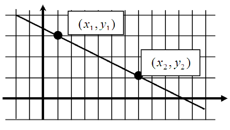
Figure 14.1: Slope between two points.
We have spent some time discussing the basic families of functions. These functions can be used to model the behavior of various real-world business situations. For example, suppose we have data based on the total cost of paying back a loan (for a fixed principal and fixed payback period). We can use this data to develop a function, call it C(r), which represents this cost as a function of different interest rates on the loan. Suppose interest rates are increasing. How will this affect the cost of paying back the loan?
This question really centers on how the function C changes as the interest rate r increases. To answer this question, we will turn to our knowledge of families of functions. In particular, we will use what we know about the parameter A in the general formula for a linear function, y = A + Bx.
Look at the graph of the linear function shown in figure 14.1. Also shown on the graph are two points. These points are labeled with the coordinates (x1,y1) and (x2,y2). What is the total change in the linear function between the two points?
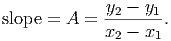
Between these points, there is a change of y2 - y1. This is just the vertical separation between the two points. Now, how quickly is the function changing at the first point? This is not a question of total change, but of the rate of change of the function. Another way of asking this question is ”If I make a small change in x from x1 to x2, how much will the function change?” To answer this question, we look at the slope of the line. As you may recall, the slope of a line can be calculated from the formula
For the function above, we see that the two points have coordinates (1, 3) and (7, 1). Thus, the slope of the line is (1 - 3)∕(7 - 1) = -2∕6 = -1∕3. The negative tells us that the function (in this case a straight line) is decreasing. This means that, as we move from left to right, the value y of the function gets smaller. There are several nice things about straight lines that we can see from this example. First, unlike nonlinear functions, the slope of a straight line is exactly the same at every single value of x. This means that the slope of the function at the first point is -1∕3 and slope at the second point is also -1∕3 and the slope at x = 249 is also -1∕3. Second, it is easy to calculate the slope of a straight line. We simply look at the change in the values of the function (the y values) and divide this by the change in the x values between the two points. This will not hold for any other family of functions.
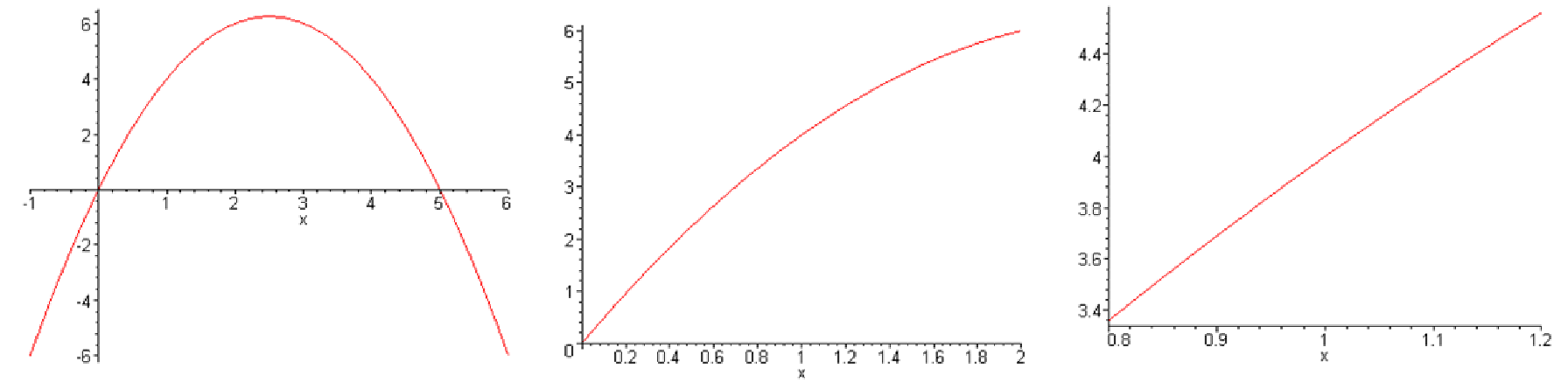
To find the slope of a nonlinear function, we take advantage of a property of smooth functions. As illustrated in the graphs in figure 14.2, if we have the graph of a nonlinear function, and we zoom in on the graph, it begins to look linear.
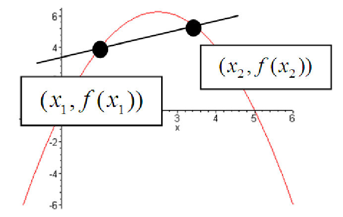
For some functions, we need to zoom in more, and for others we zoom in less to see this linear-like appearance. In order to calculate the slope, we will use this feature, called local linearity, to determine the slope of a functions at any point. Specifically, if we pick two points on the function, and draw a line between them, we will call the slope of this line the average rate of change of the function. If we call these two points (x1,f(x1)) and (x2,f(x2)), then the average rate of change between the points is
Notice that the graph in figure 14.3 shows how the average rate of change can be quite different from the actual rate of change (called the instantaneous rate of change or derivative).
However, if we move the second point closer to the first, we can get a more accurate approximation to the instantaneous rate of change of the function near the first point. If the two points are close enough, the average rate of change will be a very good approximation to the instantaneous rate of change. This fact will help us in many cases where we only have data, instead of an actual function.