14.1.2 Worked Examples

Example 14.1. Marginal Analysis with Difference Quotients
In example 1 we developed a model for the cost of electricity as a function of the number of units of electricity produced. Later in that chapter we used parameter analysis to explore how the function behaved. This analysis was all in terms of percent changes, which is somewhat limiting. In this example, we are going to use marginal analysis through the difference quotient to interpret how much each unit of electricity affects the total cost of producing the electricity. (In later examples, we will refine this process using a shortcut method called the derivative.) The cost model we will use is the square root model given by

Suppose that we are currently producing 500 units of electricity. How much would it cost to produce one more unit of electricity? We can put this into a spreadsheet to compute it fairly easily. The results are shown below, and were obtained by setting up a formula for the difference quotient of the function, with a variable for h so that we can let h get very small. This lets us see what the instantaneous rate of change of the cost function is.

From this, it seems that when current production is at 500 units, each additional unit of electricity will cost approximately $32.39. In contrast, if are currently producing 1,000 units of electricity, the marginal cost is about $22.91 per unit.

Example 14.2. Finding the Derivative of a Power Function
While it is possible to use basic algebra and the definition of the derivative (as a limit of the difference quotient) for marginal analysis this process can be tedious and will be difficult for some of the basic functions. Instead, we’re going to use trendlines to experiment to find a shortcut for the derivative of a power function. We begin with the power function f(x) = x². Here’s an outline of what we’ll do:

1. Set up a spreadsheet that has places to enter the parameters of the function (A and B).
2. Add in a place for us to enter a value for h, the number we need in the difference quotient.
3. Create columns for x and f(x) and compute the values for the column under f(x) from the values listed under the x column.
4. Next we add columns to compute x + h and f(x + h).
5. We add a column to compute the difference quotient from the data we’ve already set up.
6. Since we have lots of x values (running down the table,) we now have a bunch of points of the form (x, difference quotient of f at x). If we make a scatterplot of these points, we can fit a trendline to these data and determine the equation of the difference quotient in the process. Thus, we are close to experimentally determining an equation for the derivative function.
7. Up till now we have kept h fixed. We can then simulate the limit of the difference quotient by making h a smaller and smaller number, until we think we see what the ”real” equation would be with h equal to zero. (Note that we can’t actually set h to be zero, since we would be dividing by zero, which gives an error!)

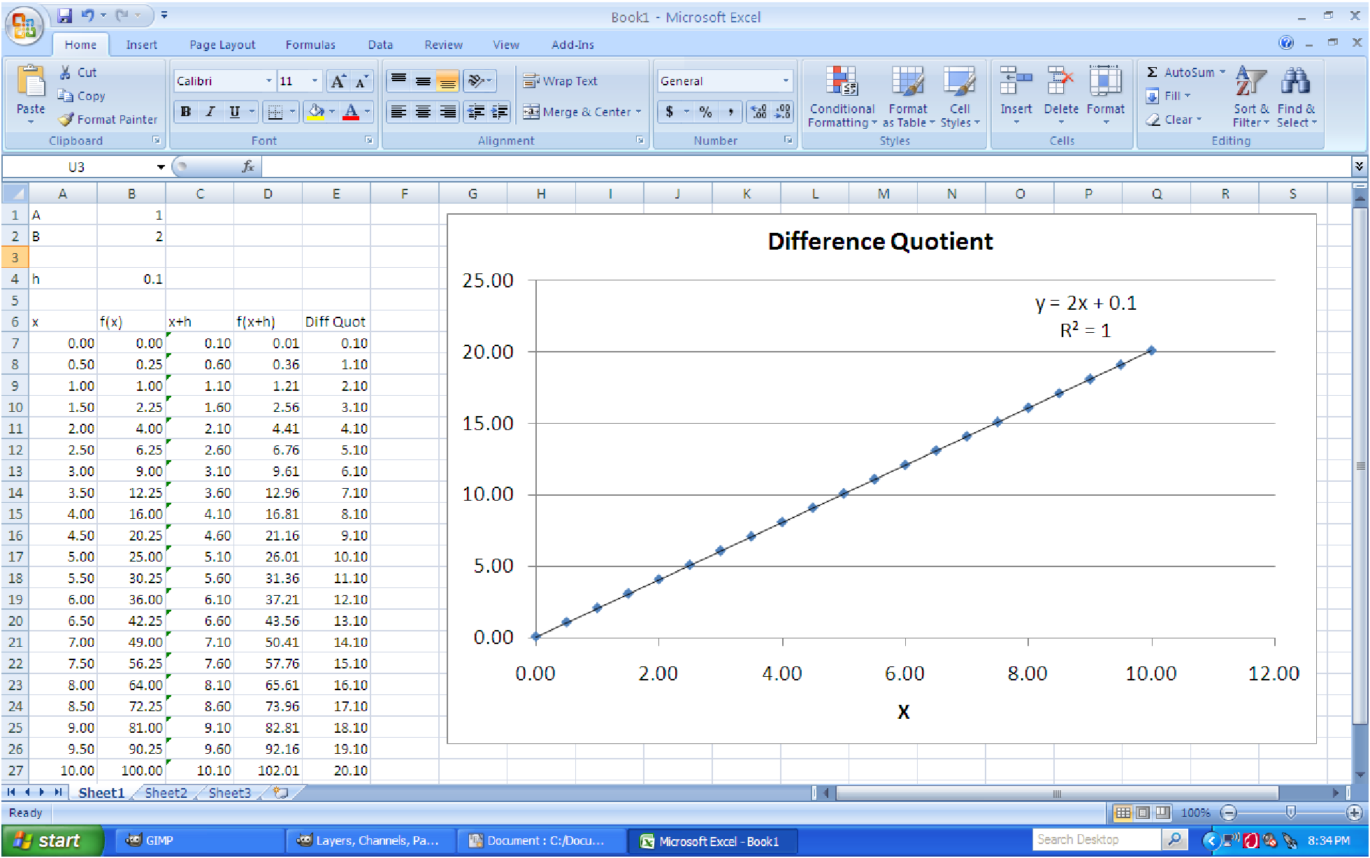
The screen shots below will show you what our spread sheet looks like at the end of this process. To go through this procedure, open the file C14 SquareDerivative.xls [.rda]. Starting with the power function

and setting h initially to 0.1, and listing x values from 0 to 10 in steps of 0.5, we get the table of data (using steps 1-6 above) shown in figure 14.6.

Now, what kind of trendline does the difference quotient make? It looks like a straight line, so let’s add a linear trendline to the graph. From this we get a fairly accurate equation:

But, we have a (mathematically speaking) pretty large value of h. Let’s vary h and collect the results of the trendline into a table like the one below. Notice that as h gets smaller, the y-intercept of the trendline decreases. Since the derivative is the limit as h goes to zero of this difference quotient, we can reasonably conjecture that as h shrinks down to zero, so does the y-intercept, leading us to the following simple rule:

The derivative of the function y = x² is the function y = 2x.

However, this only gives us the derivative of one single power function. What about all the other ones? How can we determine their derivatives without going through this fairly lengthy process every time? We’ve actually almost got the answer, since our spreadsheet is set up to allow us to change the parameters in the power function and find rules for those as well. This is what the exploration in this section is all about - finding the rules for ALL of the power functions. It turns out to be relatively simple.

Example 14.3. Marginal Analysis with Derivatives
Suppose we know that our costs for producing q thousand goods are C(q) = q², where C is measured in millions of dollars. If we are currently producing 10,000 goods, how will our costs increase if we add an additional 1,000 goods to the production?

For this situation, we are currently producing q = 10 thousand items and want to know what happens to the cost if we produce q = 11 thousand items. This is an increase of 1 (in our units of q) so it is a question about the marginal cost. Since the marginal cost is really just the derivative (slope) of the cost function, we can use the last example to help us out. In that example, we used spreadsheets, difference quotients, and regression to learn that the derivative of x² is 2x. Thus, the derivative of the cost function, denoted C′, is C′(q) = 2q and the marginal cost of producing 10,000 goods is C′(10) = 2(10) = 20. The units of the derivative are (units of function/units of independent variable) so the complete answer is:

This means that if we want to increase production to 11,000 goods, we can expect an increase in the costs of about 20 million dollars. If we wanted to produce 12,000 goods the cost would increase by approximately ($20 million per thousand goods) ⋅ (2 thousand goods) = 40 million dollars (since 12,000 is 2,000, or 2 thousands, greater than 10,000.) If, on the other hand, we decrease the production to 9,500 goods, then the cost will change by about ($20 million per thousand goods) ⋅ (-0.5 thousand goods) = -10 million dollars. (The negative sign simply means that the cost decreases if we decrease production.)