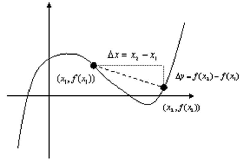
Note that the order is important! If you start with x2 first in the numerator, you must also start with x2 in the denominator. The graph below shows the basic idea and illustrates why it’s called average slope and not the actual slope. The dashed line between the two points represents the average slope of the function (the curved line) between those two points. In between the two points, though, notice that there are places where the curve has a more negative slope than the average slope and places where the slope is even positive!
Consider the line passing through the point (x1,f(x1)) and having the same slope as the difference quotient, with a fixed value of h, say 1. If we look at this line for smaller and smaller values of h (say 0.1, 0.01, 0.001, etc.) we see that the line eventually becomes ”parallel” with the function at the point (x1,f(x1)). This visual process of watching the line become parallel can be carried out mathematically through a limit.
How much bang do I get for each additional buck that I spend?
 which indicates that we are interested in the slope of f in the x-direction.
Thus, a positive number for the derivative means that as x increases (we always
move to the right) the value of f is increasing. Likewise, a negative value of the
derivative indicates that the function is decreasing at that point. Officially, the
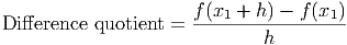
derivative of a function at a point is computed by taking the difference quotient and
letting h go to zero. This is noted mathematically by the ”limit of the difference
quotient”:
which indicates that we are interested in the slope of f in the x-direction.
Thus, a positive number for the derivative means that as x increases (we always
move to the right) the value of f is increasing. Likewise, a negative value of the
derivative indicates that the function is decreasing at that point. Officially, the
derivative of a function at a point is computed by taking the difference quotient and
letting h go to zero. This is noted mathematically by the ”limit of the difference
quotient”:
![[ ]
f(x + h ) - f (x )
f′(x) = lim ----------------
h→0 h](Text_Fall_2014259x.png)
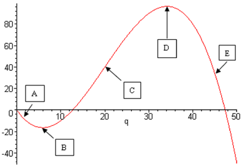
 . Since the derivative tells how fast the function is
changing, the second derivative tells us how fast the first derivative is changing. Thus, it
measures the rate of change of the slope, which is called concavity. In a graph, concavity is
easy to see: it refers to the direction and steepness of the way the function bends. If it bends
up (looks like a cup) then the concavity is positive. If it bends down (looks like a frown) then
the concavity is negative. If the function is almost flat, then the concavity is close to
zero.
. Since the derivative tells how fast the function is
changing, the second derivative tells us how fast the first derivative is changing. Thus, it
measures the rate of change of the slope, which is called concavity. In a graph, concavity is
easy to see: it refers to the direction and steepness of the way the function bends. If it bends
up (looks like a cup) then the concavity is positive. If it bends down (looks like a frown) then
the concavity is negative. If the function is almost flat, then the concavity is close to
zero.