Worked Examples

17.2.2 Worked Examples

Example 17.4. Future Value of an Income Stream

Let

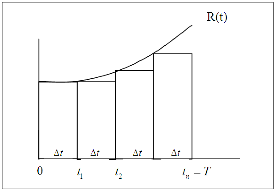
R(x) = Rate of income at time t r = Interest rate compounded continuously T = Number of years the income stream is invested

We divide the interval [0,T] into n subintervals of length Δt = Tn- and create n rectangles under the R(x) as seen in the figure below.

Figure 17.4: Using integration to find the future value of an income stream.

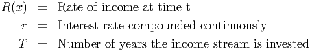
The height of the ith rectangle is R(t_i) and its width is Δt. R(t_i)Δt, the area of the ith rectangle, is the approximately the amount of the income stream to be invested between t_i-1 and t_i. If we think of investing this small principal at the continuous rate r for a period of T -t_i years (this is the remaining time for the investment from t_i to T), then the amount that will be accumulated after T years is [R(t_i)Δt]e^r(T-t_i). This formula is derived from the compound interest formula A = Pe^rt (see example 4) where P = R(t_i)Δt and e^rt is replaced by e^r(T-t_i). Therefore, the Riemann sum of the future values of the areas of the rectangles is

r(T -t1) r(T-t2) r(T-t3) r(T- tn) [R (t1)Δt]e + [R (t2)Δt ]e + [R (t3)Δt ]e + ...+ [R (tn)Δt ]e = [R (t1)Δt ]erT e-t1 + [R (t2)Δt ]erTe- t2 + [R (t3)Δt]erTe-t3 + ...+ [R(tn)Δt ]erTe- tn

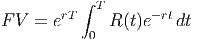
Factoring out e^rT and Δt, we have

rT [ -t1 -t2 -t3 - tn] = e [R (t1)]e + [R (t2)]e + [R (t3)]e + ...+ [R (tn)]e Δt

Letting n →∞, we have the following result:

The future value after T years of an income stream R(t) dollars per year, invested at the rate r per year compounded continuously, is

rT ∫ T -rt F V = e 0 R (t)e dt

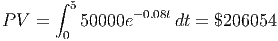
To illustrate this idea, consider Glow Health Spa. Glow Health Spa recently bought a full-body dermal treatment machine that is expected to generate $50,000 in revenue per year for the next 5 years. If this income stream is invested at 8% per year compounded continuously, what is the future value of this income stream in 5 years?

R(t)	= 50,000 where t is in years
	Note: the income stream R(t) is a constant amount per year in this example.
r	= .08
T	= 5 years
Future Value	= e^0.08(5) ∫₀⁵50000e^-0.08t dt = 1.49 ∫₀⁵50000e^-0.08t dt
	= 1.49(206054)=$307,020
	where the definite integral is calculated using the Basic Integration Tool.

Example 17.5. Present Value of an Income Stream
The present value of an income stream of R(t) dollars per year over T years, earning interest at the rate of r per year compounded continuously, is the principal P that would have to be invested now to yield the same accumulated value as the investment stream would earn if it were invested on a continuing basis for T years at rate r.

In equation form, we have

∫ T PerT = erT R(t)e-rtdt. 0

Dividing both sides of this equation by e^rT, we have PV = ∫₀^TR(t)e^-rt dt, the present value of the income stream R(t).

To illustrate the present value of an income stream, we will consider the present value of Health Glow’s income stream (see above).

∫ 5 P V = 50000e -0.08tdt = $206054 0

Where we have used the Basic Integration Tool in the last step. This means that in order to equal the future value ($307,020) of investing an income stream of $50000 for a period of 5 years at 8% compounded continuously, Health Glow would have to invest a lump sum now of $206054 for the same time period at the same rate of interest.

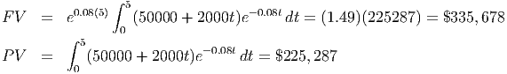
Health Glow’s revenue stream was constant ($50000) over the five-year period. Revenue streams need not be constant, however. Suppose Health Glow generated an increasing income stream given by R(t) = 50, 000 + 2000t. We find the future value and present value of this income stream as follows:

∫ 0.08(5) 5 -0.08t F V = e 0 (50000 + 2000t)e dt = (1.49)(225287) = $335, 678 ∫ 5 P V = (50000 + 2000t )e- 0.08tdt = $225,287 0

Example 17.6. Consumer Surplus
Let

p = D(x)	be the demand function for a commodity
p	the established market price of the commodity
x	the number of items sold at (i.e. the consumer demand at p)

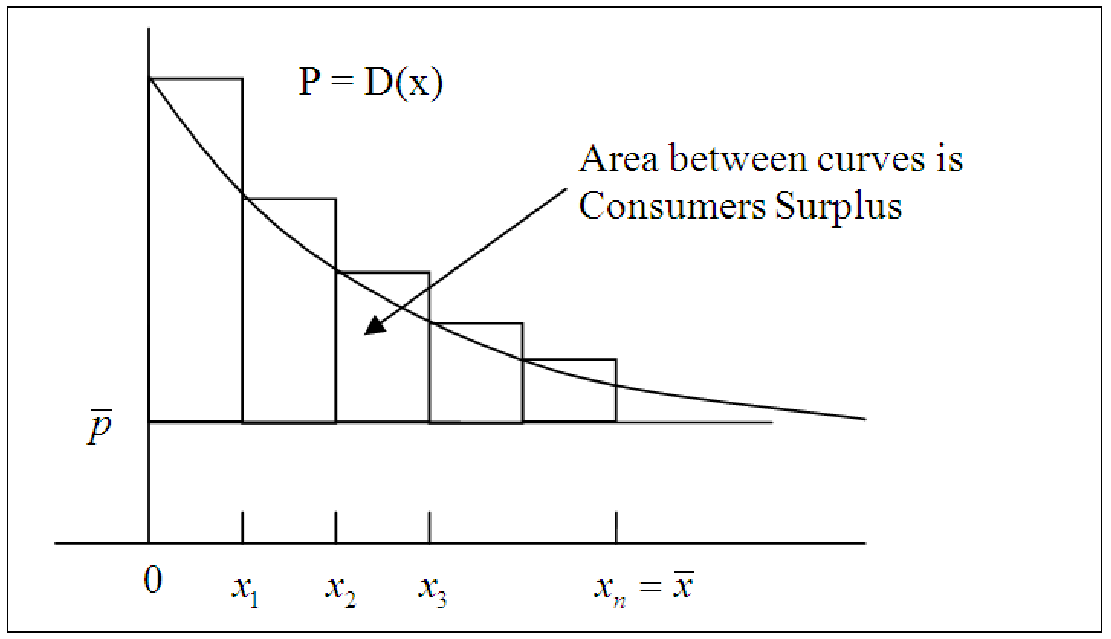
Consumers’ surplus is the difference between what consumers would be willing to pay p and the actual price p they pay. If we plot p = D(x) and the straight line p = p on the same axes, then the consumers’ surplus is the area between D(x) and p = p, i.e. D(x) -p, from 0 to x.

We find the approximate area between the two curves (the straight line p = p is considered to be a curve) by placing rectangles between them (see the figure below). The height of each rectangle is D(x) -p and the width is Δx. The area of the ith rectangle is [D(x) -p]Δx.

Figure 17.5: Integrating to compute the area between the demand curve p = D(x) and the curve p = p, the established market price of a commodity, determines the consumer surplus.

The approximate area between the curves is the Riemann sum

n ∑ [D (x ) - ¯p]Δx = [D (x ) + D (x ) + ...+ D (x )]Δx - [¯pΔx + ¯pΔx + ...+ ¯pΔx ] i=1 i 1 2 n ◟-----------◝◜----------◞ n terms add to p¯(n Δx ) = ¯p¯x because nΔx = ¯x

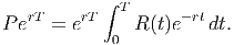
Taking the sum as n →∞, we have

∑n ∑n ∫ ¯x lim [D (xi) - ¯p]Δx = lim D (xi)Δx = D (x )dx - ¯p¯x n→∞ i=1 n→∞ i=1 0

So, CS = ∫ ₀^xD(x) dx-px. To illustrate this concept, suppose the demand function is given by P = D(x) = -0.01x² - 0.3x + 25 where

p	is the wholesale price in dollars
x	is the demand in thousands
p = 10	the established market price (in dollars)

We need to find the intersection of p = D(x) and p = 10 in order to find the area between the two curves. See the figure below.

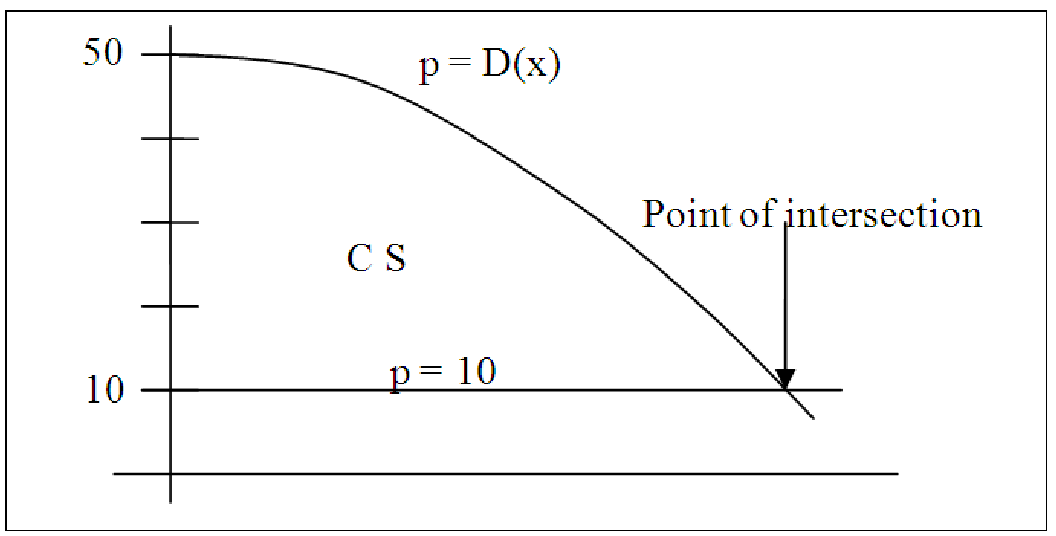
Figure 17.6: Finding the point of intersection to determine the limits of integration for computing consumer surplus.

Using Goal Seek in Excel or uniroot in R, we find the demand at $10 is x ≈ 26 (rounded down to the nearest whole number). Substituting in the formula above and using the Basic Integration Tool for the definite integral, we have

∫ 26 (- 0.01x2 - 0.3x + 25 )dx - (10)(26) = 500 - 260 = $240 thousand 0

Example 17.7. Producers’ surplus
Let

p = S(x)	be the supply function for a commodity
p	be the established market price of the commodity
x	be the number of items producers are will to supply at p (i.e. the consumer demand at p)

The producers’ supply is the difference between what the suppliers actually receive and what they are willing to receive. The producers’ surplus is the area between the line p = p and the supply curve S(x).

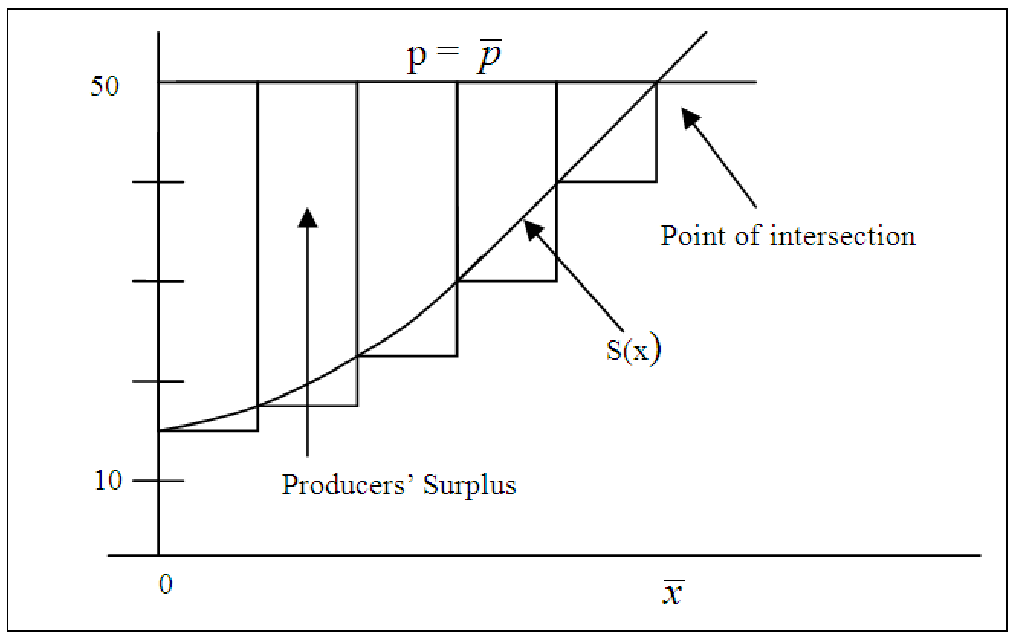
Figure 17.7: Using integration to find producer surplus, the area between the fair maarket price curve p = p and the supply curve p = S(x).

Similar to what we did for the consumers’ surplus, we find the area between the two curves to be the definite integral

∫ ¯x Producers ’ Surplus = p¯¯x - S(x )dx 0

To illustrate this concept, suppose the supply function is given by P = S(x) = 0.1x² + 3x + 15 where

p	is the price in dollars
x	is the demand in thousands
p = 50	is the established market price

Before we can find the Producers’ Surplus = px-∫ ₀^xS(x) dx, we need to find the intersection of p = 50 and p = S(x) in order to find the area between the two curves. Using Goal Seek in Excel or uniroot in R, we find the demand at $50 is x ≈ 9. Substituting into the formula above and using the Basic Integration Tool for the definite integral, we have

∫ 9 2 (50)(9) - (0.1x + 3x + 15)dx = 450 - 281 = $169 thousand 0

[next] [prev] [prev-tail] [front] [up]