9.1.1 Definitions and Formulas

Multiple linear function

This is a model much like a normal linear model, except that it includes several explanatory variables. If the explanatory variables are labeled X₁, X₂, … and the response variable is Y , then a multiple-linear model for predicting Y would take the form

Notice that the multiple linear function has a ”y-intercept” given by A. Each of the coefficients (the B_i’s) is a slope associated with one of the explanatory variables.

An important difference between linear and multiple linear models is the graphical illustration of each. A linear function describes a line in two dimensions. A multiple linear function with two explanatory variables describes a plane in three-dimensional space. If there are more than two explanatory variables, we cannot picture the ”hyperplane” that the function describes.

Multiple linear regression

The process by which you can ”least squares fit” a multiple linear function to a set of data with several explanatory variables.

Stepwise regression

This is an automated process for determining the best model for a response variable, based on a given set of possible explanatory variables. The procedure involves systematically adding the explanatory variables, one at a time, in the order of most influence. For each variable, a p-value is determined. The user controls a cut-off for the p-values so that any variable with a p-value above the cut-off gets left out of the model.

p-values

A p-value is a probability assigned to determine whether a given hypothesis is true or not. In regression analysis, p-values are used to determine whether or not a given explanatory variable should have a coefficient of ”0” in the regression model. If the p-value is above 0.05 (5%) then one can usually leave the variable out and get a model that is almost as good.

p < 0.05	Keep the variable
p > 0.05	Drop the variable

Controlling variables

This is the process by which the person modeling the data tries to account for data which may have several observations that are similar in some variables, but differ in others. For example, in predicting salaries based on education, you should control for experience, otherwise the model will not be very accurate, since several employees may have the same education, but different salaries because they have different experience.

Degrees of Freedom for Multiple Regression Models

In multiple regression models, one is usually estimating several characteristics of the population that underlies the data. For each of these estimated characteristics, one degree of freedom is lost. If there are n observations, and you are estimating a multiple regression model with p explanatory variables, then you loose p + 1 degrees of freedom. (The ”+1” is for the y-intercept.) Thus,

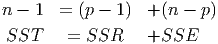
Also notice that in the ANOVA table for multiple regression, the degrees of freedom of the Explained (p - 1) plus the degrees of freedom of the Unexplained (n - p) add up to the degrees of freedom of the sum of the squares of the total variation (n - 1):

(Total Variation = Sum of Squares of Unexplained + Sum of Squares of Explained)

Multiple R²

This is the coefficient of multiple determination used to determine the quality of multiple regression models.

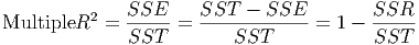
SSR=	Sum of the squares of the residuals (unexplained variation)
SSE =	Explained amount of variation
SST =	Total variation in y

Multiple R² is the coefficient of simple determination R-Squared between the responses y _i and the fitted values ŷ_i.

A large R² does not necessarily imply that the fitted model is a useful one. There may not be a sufficient enough number of observations for each of the response variables for the model to be useful for values outside or even within the ranges of the explanatory variables, even though the model fits the limited number of existing observations quite well. Moreover, even though R² may be large, the Standard Error of Estimate (S_e) might be too large for when a high degree of precision is required.

Multiple R

This is the square root of Multiple R². It appears in multiple regression output under ”Summary Measures”.

Adjusted R²

Adding more explanatory variables can only increase R², and can never reduce it, because SSE can never become larger when more explanatory variables are present in the model, while SSTO never changes as variables are added (see the definition of multiple R² above). Since R² can often increase by throwing in explanatory variables that may artificially inflate the explained variation, the following modification of R², the adjusted R², is one way to account for the addition of explanatory variables: This adjusted coefficient of multiple determination adjusts R² by dividing each sum of squares by its associated degrees of freedom (which become smaller with the addition of each new explanatory variable to the model):

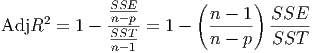
The Adjusted R² becomes smaller when the decrease in SSE is offset by the loss of a degree of freedom in the denominator n - p.

Full Regression Model

The full regression model is the multiple regression model that is made using all of the variables that are available.