| Regression Coefficients
| |
| Coefficient | |
| Constant | A |
| X1 | B1 |
| X2 | B2 |
| X3 | B3 |
 |  |
Example 9.1. Reading multiple regression output and generating an equation
In the last chapter, if you did the memo problem, you have encountered Ms. Carrie Allover, who
needed help determining how each of the possible variables in her data are related to the number of
riders each week on the commuter rail system she runs for a large metropolitan area. (See data file
C09 Rail System.xls [.rda].) However, in the last chapter, we were forced to examine the data
one variable at a time. Now, we can try to build a model that incorporates all of the variables,
so that each is controlled for in the resulting equation. If we produce a full regression
model using the numerical variables, we get the following output. But what does it
mean?
| Results of multiple regression for Weekly Riders
| |||||||
|
| |||||||
| Summary measures | |||||||
|
| Multiple R | 0.9665 | |||||
|
| R-Square | 0.9341 | |||||
|
| Adj R-Square | 0.9259 | |||||
|
| StErr of Est | 23.0207 | |||||
|
| |||||||
| ANOVA table | |||||||
|
| Source | df | SS | MS | F | p-value | |
|
| Explained | 4 | 240471.2479 | 60117.8120 | 113.4404 | 0.0000 | |
|
| Unexplained | 32 | 16958.4277 | 529.9509 | |||
|
| |||||||
| Regression coefficients | |||||||
|
| Lower | Upper | |||||
|
| Coefficient | Std Err | t-value | p-value | limit | limit | |
|
| Constant | -173.1971 | 220.9593 | -0.7838 | 0.4389 | -623.2760 | 276.8819 |
|
| Price per Ride | -139.3649 | 42.7085 | -3.2632 | 0.0026 | -226.3593 | -52.3706 |
|
| Population | 0.7763 | 0.1186 | 6.5483 | 0.0000 | 0.5349 | 1.0178 |
|
| Income | -0.0309 | 0.0106 | -2.9233 | 0.0063 | -0.0524 | -0.0094 |
|
| Parking Rate | 131.0352 | 33.6529 | 3.8937 | 0.0005 | 62.4866 | 199.5839 |
First of all, you will notice that the regression output is very similar to the output from simple regression. In fact, other than having more variables, it is not any harder to develop the model equation. We start with the response variable, WeeklyRiders. We then look in the ”Regression Coefficients” for each coefficient and the y-intercept. The regression coefficients are in the format:
| Regression Coefficients
| |
| Coefficient | |
| Constant | A |
| X1 | B1 |
| X2 | B2 |
| X3 | B3 |
| | |
From this, we can easily write down the equation of the model by inserting the values of the coefficients and the names of the variables from this table into the multiple regression equation shown on page 480:

Example 9.2. Interpreting a multiple regression equation and its quality
The rail system model (previous example, see the data file C09 Rail System.xls [.rda]) can be
interpreted in the following way:
How good is this model for predicting the number of weekly riders? Let’s look at each summary measure, then the p-values, and finally the diagnostic graphs. The R2 value of 0.9341 indicates that this model explains 93.41% of the total variation in ”weekly riders”. That is an excellent model. The standard error of estimate backs this up. At 23.0207, it indicates that the model is accurate at predicting the number of weekly riders to within 23,021 riders (at the 68% level) or 46,042 (at the 95% level). Given that there have been an average of 1,013,189 riders per week with a standard deviation of 84,563, this model is very accurate. The adjusted R2 value is 0.9259, very close to the multiple R2. This indicates that we shouldn’t worry too much about whether we are using too many variables in the model. When adjusted R2 is really different from the R2, we should look at the variables and see if any can be eliminated. In this case, though, we should keep them all, unless either the p-values (below) tell us to eliminate a variable or unless we just want to build a simpler, easier-to-use model.
Are there any variables included in the model which should not be there? To answer this, we look at the p-values associated with each coefficient. All but one of these is below the 0.05 level, indicating that these variables are significant in predicting the number of weekly riders. The only one that is a little shaky is the y-intercept. It’s p-value is 0.4389, far above the acceptable level. This means that we could reasonably expect that the y-intercept is actually 0, and that would make a lot of sense in interpreting the model. Given this high p-value, you could try systematically eliminating some of the variables, starting with the highest p-values, and looking to see if the constant ever becomes significant.
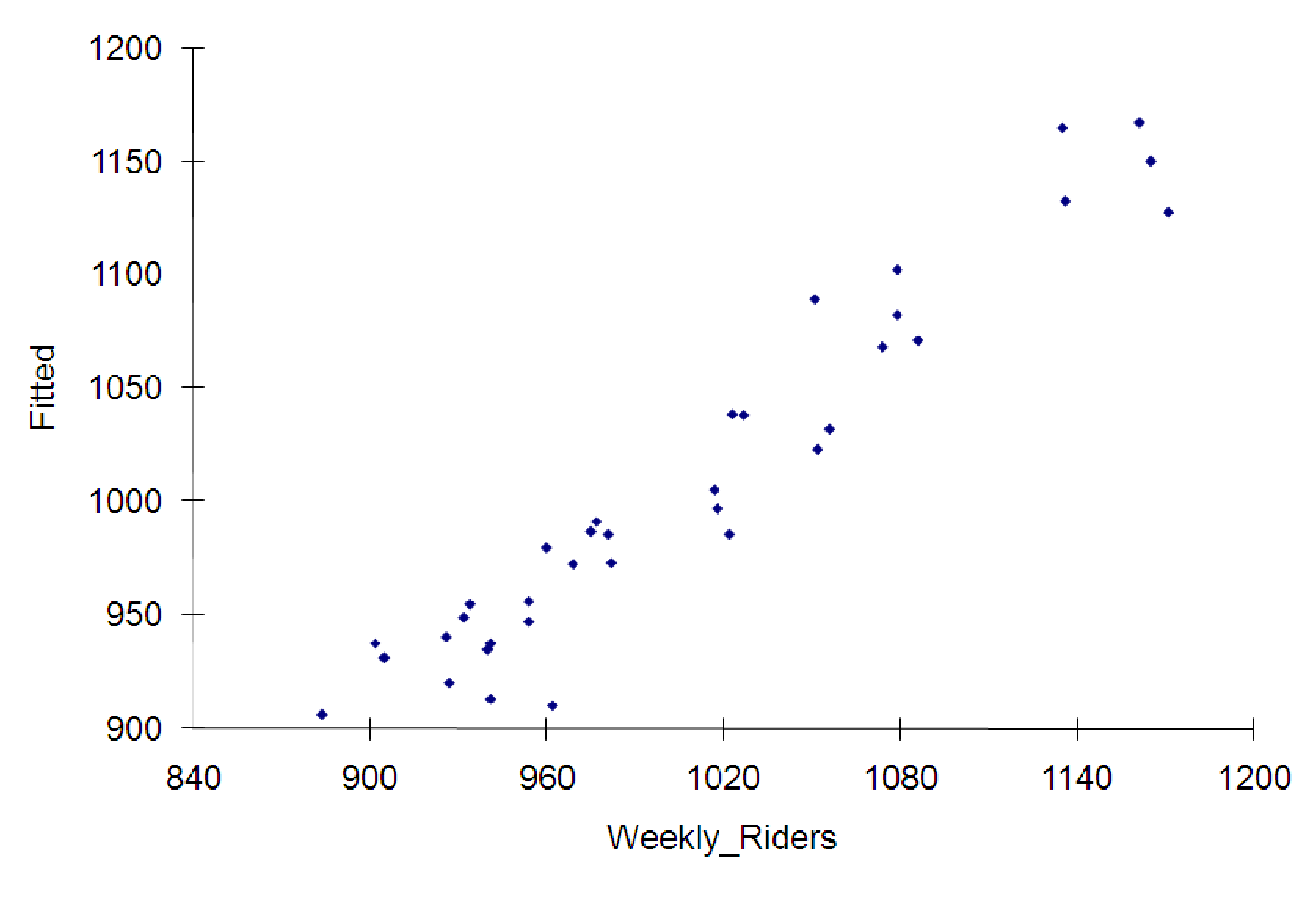
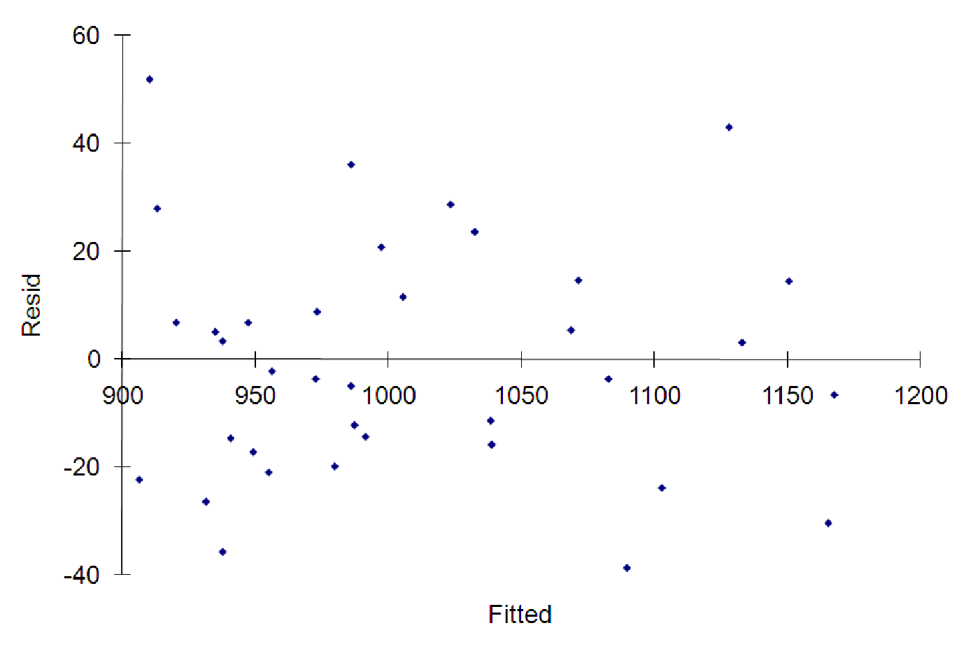
What about the diagnostics graphs? We have four explanatory variables, so we cannot graph the actual data to see if it is linear. Our only options involve the ”Fitted vs. Actual” and the ”Residuals vs. Fitted” graphs that the software can produce. These graphs are shown below.
In the ”fitted vs. actual” graph, we see that most of the points fall along a straight line has a slope very close to 1. In fact, if you add a trendline to this graph, the slope of the trendline will equal the multiple R2 value of the model! So far, it looks like we’ve got an excellent model for Ms. Carrie Allover.
In the ”residuals” graph, we are hoping to see a random scattering of points. Any pattern in the residuals indicates that the underlying data may not be linear and may require a more sophisticated model (see chapters 10 and 11). This graph looks pretty random, so we’re probably okay with keeping the linear model.
Example 9.3. Using a multiple regression equation
Once you have a regression equation, it can be used to either
Suppose, for example, that Ms. Allover (see the data file C09 Rail System.xls [.rda]) wants to use the regression model that we developed above to predict what next year’s weekly ridership will be. If we know what the population, disposable income, parking costs, and price per ride are, we can simply plug these into the equation to calculate the number of weekly riders. Our data stops at 2002. If we know that next year’s ticket price won’t change, and that the economy is about the same (so that income and parking costs stay the same in 2003 as in 2002) then all we need to know is the population. If demographics show that the population is going to increase by about 5% in 2003, then we can use this to calculate next year’s weekly ridership:
Next year’s population = (1 + 0.05)*Population in 2002 = 1.05*1,685 = 1,770
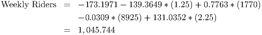
It is important to notice that if any of the variables change, the final result will change. Also notice that a 5% change in population while keeping all the other explanatory variables constant results in a (1045.744 - 960)/960 = 8.9% change in the number of weekly riders. If the values of the other variables were different, the change in the number of weekly riders would be a different amount.
If we wanted to solve the regression equation for values of the explanatory variables, keep in mind this rule: For each piece of ”missing information” you need another equation. This means that if you are missing one variable (either weekly riders, price per ride, population, income, or parking rates) then you can use the values of the others, together with the equation, to find the missing value. If you are missing two or more variables, though, you need more equations.