Definitions and Formulas

Any model relating two variables (say x and y) in such a way that changes in one variable are not in a constant ratio to the changes in the second variable is said to be non-proportional. Another way of describing this is by saying that there is no constant k for which the following relation is true:

y2 - y1 = k(x2 - x1)

In the mathematical world and in the real world, most models are non-proportional.

Any model that is level dependent is also said to be non-proportional. The term level-dependent emphasizes that with such models, the amount that the y variable increases for a given increase in x is different if the starting point (x value or location along the horizontal axis) is moved. In other words, you can look at different x and y values and compute their differences. When we compare them, if we find that y₂ - y₁ = k₁₂(x₂ - x₁) and y₄ - y₃ = k₃₄(x₄ - x₃), but the k values are different, then the model is level-dependent and represents a non-proportional relationship.

Concavity is a property of non-proportional models. It refers to the amount that the graph of the model bends. If the graph bends upward, that part of the graph is said to be ”concave up”. If the graph bends downward in a certain area, then the graph is ”concave down” in that area. Remember: concave up looks like a cup; concave down looks like a frown.

One of the six functions listed below as prototypes for fitting nonlinear data:

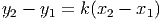
linear,
logarithmic,
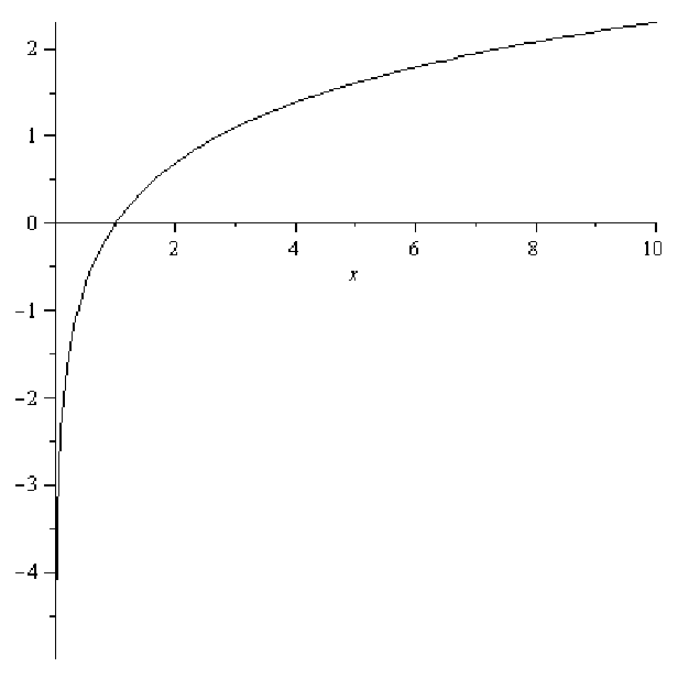
exponential,
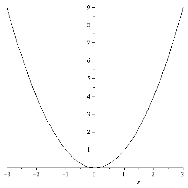
square,
square root, or
reciprocal.

In general, a function is a mathematical object that takes an input, usually in the form of a number or a set of numbers, and gives an output number. (There are other types of functions possible, but we will concentrate on functions that satisfy this definition.) For a relationship between two variables, say x and y, to be a function, it must satisfy the following statement:

Every x-value must be associated with one and only one y-value.

This means that if you draw a graph of the function, and draw a vertical line through any point on the graph, that line will only touch the graph once. This is sometimes referred to as the vertical line test. Generally, if the variable y is a function of the variable x, we write y = f(x) to indicate this. If the variable y is a function of several variables (say x₁, x₂, x₃) then we write y = f(x₁,x₂,x₃).

Graphs of linear functions (see figure 11.1) are straight lines. The prototypical, or base, form of a linear function that related y to x is given by y = x. You are more used (by this point) to seeing this in a more general form, involving two parameters, the slope and y-intercept: y = A + Bx. The graph of a linear function is shown below. Notice that linear functions are straight; they have no concavity at all.

Figure 11.1: The basic linear function y = x.

A logarithm (see figure 11.2) is a mathematical function very useful in scaling data that spans a large range of values, like from 1 to 1,000,000 (we will see this aspect of logarithms in a later chapter). In general, there are lots of different logarithmic functions. We will be using the natural logarithm of x as a function; this is written as y = ln(x). (Notice: natural logarithm = nl → ln.) The graph of the basic natural logarithm is shown below. The basic logarithm is increasing and concave down everywhere.

Figure 11.2: The basic logarithmic function y = ln(x).

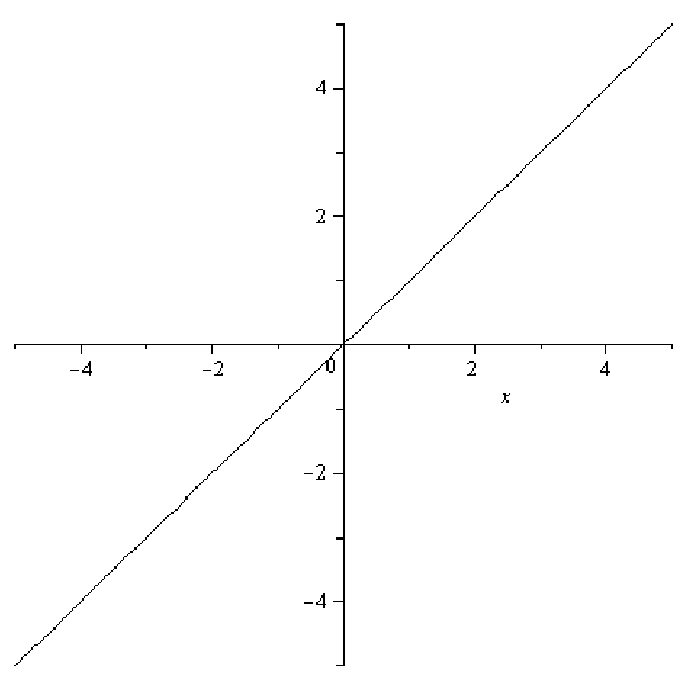
The natural logarithmic function has several important properties to note. The natural log of 0 is undefined; in other words ln(0) does not exist. If 0 < x < 1 then ln(x) < 0, and ln(1) = 0. This means that the point (1, 0) is common to all basic log functions. This is actually a restatement of the fact that any base raised to the zero power is equal to 1.

Exponential functions (see figure 11.3) are related to logarithmic functions. These can be written in two ways. The first form is as a base number raised to a variable power (y = a^x). The most common base to use is the number e, which is approximately 2.71828… In reality, e is an irrational number, like π. It shows up naturally in many situations, as we will see in example 4 from chapter 15 when examining interest rates. For now, though, the standard exponential function we will use is y = e^x. The second form is similar to this, but easier to type: y = exp(x). This can be read as ”y is the exponential function of x” or ”y equals e raised to the x power.” Its graph is shown below. The basic exponential function is increasing and concave up everywhere.

Figure 11.3: The basic exponential function y = exp(x).

In addition, since any positive number, like e, raised to a negative power is a number between 0 and 1, we know that if -∞ < x < 0 then 0 < e^x < 1. Since any number raised to the zero power is 1, we also know that e⁰ = 1 so the point (0, 1) is on the graph of all basic exponential functions.

You are probably familiar with the squaring function: it takes every number put into it and spits out that number raised to the second power. Thus, if we stick in the number x, we get out x². Thus, the basic squaring function is y = x². The graph of this function has a special name that you may have heard before: a parabola. It looks like the letter ”U”, centered at (0, 0). The basic squaring function is concave up everywhere. as shown in figure 11.4.

Figure 11.4: The basic squaring function y = x².

The square root function does the opposite of what the squaring function does. This function takes in a number and spits out its square root. The square root of a number is that number which, when squared, produces the number. For example, 2 is the square root of 4, since 2 × 2 is 4. The square root function is usually written as y = √--
x

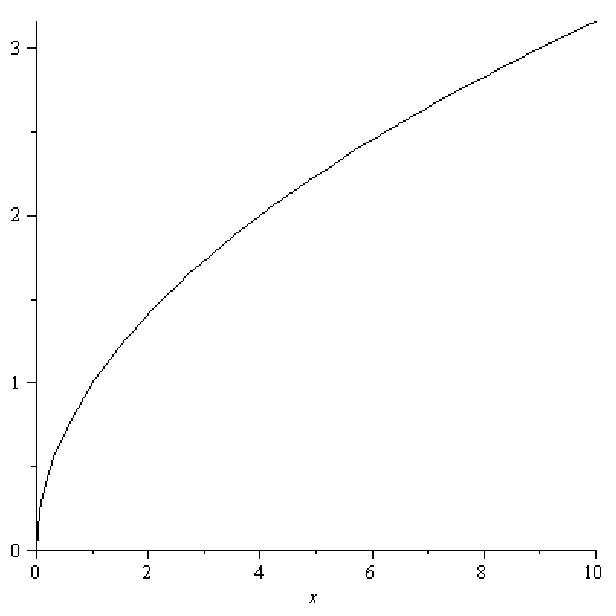
. Another way to write the function reminds us of its relationship with the squaring function: y = x^1∕2 = x^0.5. (Read this as: y is x raised to the one-half power or x to the 0.5 power.) The basic square root function is concave down everywhere. In figuer 11.5, the square root function is not graphed for values of x less than 0, since the square root of a negative number is an imaginary quantity.

Figure 11.5: The basic square root function y = √ --
x

.

The reciprocal function takes a number and returns one divided by that number: y =

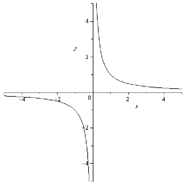
. This function also has an alternative form in which x is raised to a power: y = x^-1. Notice that the reciprocal function shown in figure 11.6 has several interesting features: It has different concavity on the left and the right; it does not even exist at x = 0 since any number divided by zero is undefined; in fact, the reciprocal function never crosses either axis.

Figure 11.6: The basic reciprocal function y = x^-1 = 1
x

.

11.1.1 Definitions and Formulas