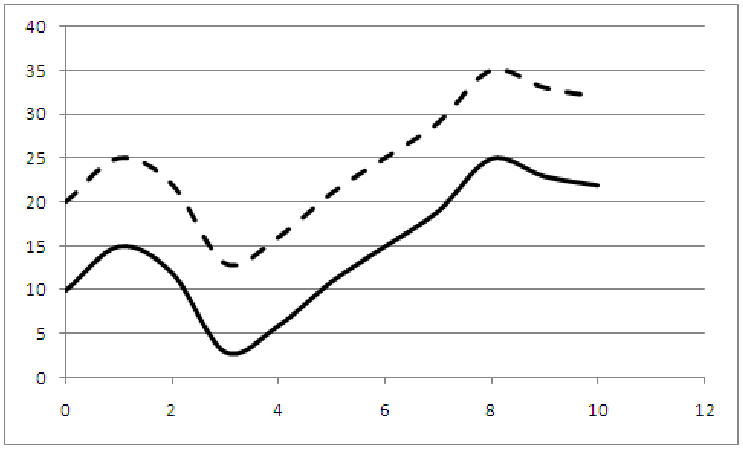
Figure 11.13: Graph of y = f(x) (solid line) and y = f(x) + 10 (dashed line).
Example 11.4. Vertical shift
Consider the data shown in the table below for y = f(x). If we make a new function by
adding the same amount, say 10, to each of these y values, then we will be creating
the function y = f(x) + 10; each y value will be 10 more than it would be without
the increase. This will result in the graph of the function being shifted up by 10 units
at each data point. It’s just like we picked up the graph and slid it up the y-axis 10
units.
| x | y = f(x) | y = f(x) + 10 |
| 0 | 10 | 20 |
| 1 | 15 | 25 |
| 2 | 12 | 22 |
| 3 | 3 | 13 |
| 4 | 6 | 16 |
| 5 | 11 | 21 |
| 6 | 15 | 25 |
| 7 | 19 | 29 |
| 8 | 25 | 35 |
| 9 | 23 | 33 |
| 10 | 22 | 32 |
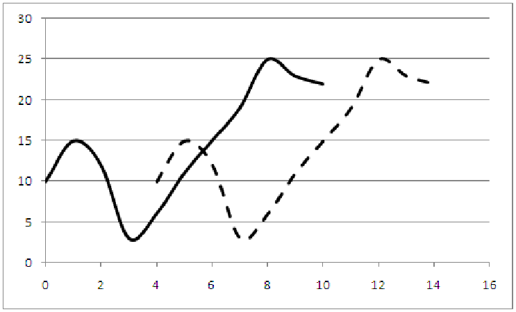
Example 11.5. Horizontal shift
We can also shift a graph to the left or right. In the last example, we added a value to all the y
values in order to shift the graph up or down the y-axis. To shift left and right, we need to add or
subtract from the x values. For example, suppose we wanted to move the graph four units to the
right. The old graph would have the point (x,y) corresponding to the statement that y = f(x).
The new graph should have the point (x + 4,y). So if the old graph had the point (3, 3), the new
graph should have the point (3 + 4, 3) or (7, 3). Here’s the catch, though, the function will only give
3 for y if we plug in a value of 3 for x. We want to plug in 7 for x and get 3 out. Thus, we
need to subtract 4 from each x value in order to make sure the function gives the right
output. This means that to shift the function to the right 4 units, we need to plot the
graph of y = f(x - 4). This is shown in the data table below and the graph beside
it.
| x | y = f(x) | y = f(x - 4) |
| 0 | 10 | ? |
| 1 | 15 | ? |
| 2 | 12 | ? |
| 3 | 3 | ? |
| 4 | 6 | 10 |
| 5 | 11 | 15 |
| 6 | 15 | 12 |
| 7 | 19 | 3 |
| 8 | 25 | 6 |
| 9 | 23 | 11 |
| 10 | 22 | 15 |
| 11 | ? | 19 |
| 12 | ? | 25 |
| 13 | ? | 23 |
| 14 | ? | 22 |
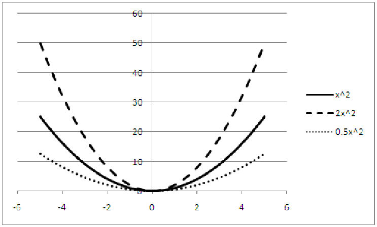
Example 11.6. Vertical scaling
We can also stretch the shape of a graph out. Suppose that we have a set of data that looks
parabolic, so we want to use the square function. But suppose that the data contains the points
(1, 1), (2, 8), (3, 18), and (4, 32). For a basic squaring function, this can’t happen; the shape is
right, but 2 × 2 = 4, not 8; 3 × 3 = 9, not 18; and 4 × 4 = 16, not 32. But notice,
that each of the actual data values is simply twice what the squaring function would
give. Thus, we want to graph y = 2x2. This means that we should take each value of x,
compute x2, and then multiply the result by 2. This stretches the graph out to fit the
data.
We can also compress a graph, squashing it down flatter instead of stretching it up taller. Suppose that the data contains the points (1, 0.5), (2, 2), (3, 4.5) and (4, 8). Each of the y values is half of what we would expect from the squaring function, so we want to graph y = 0.5x2. We see that the general form to scale the graph of y = f(x) is y = a × f(x) where a is a constant. The graphs below show the basic squaring function and the two functions we have just created.
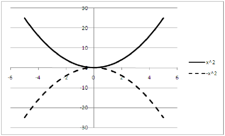
But what happens if we let a be a negative number? This will simply take each of the old y values from the function and put a negative sign in front of them. This flips the graph over the x-axis, creating a mirror reflection of the original graph. Thus, the graph of y = -f(x) is the same as the graph of y = f(x) except that it is flipped over the x-axis. In a similar way, multiplying x by a factor can scale the graph horizontally, and negating x flips the graph horizontally over the y-axis.
Example 11.7. Combination of Shifts and Scales
Consider the graphs shown in the introduction to this section in figure 11.11. The data for the
number of motors returned as a function of inspection expenditures looks to be a basic squaring
function, but shifted and scaled. Here’s another look at the graph.
It looks like the graph has been shifted to the right 60 units and up 64 units. Thus, we could start by comparing the data to the graph of y = f(x- 60) + 64 = (x- 60)2 + 64. When we do this, we find that the graph starts in the right place, but climbs too quickly. We might be tempted to simply multiple this whole thing by a constant less than one in order to squash the graph, but this would also multiply the vertical shift by the constant, changing the starting place. We must complete the shifts and scaling in the proper order. We need to construct the fit by first shifting right, then scaling, then shifting. So, we are looking for a function of the form y = af(x - 60) + 64 = a(x - 60)2 + 64.
How much should we squash the graph? In other words, how big is a? The best approach here is to try a few data points. It looks like the point (80, 68) is on the graph. Plugging these values in for x and y we get the following:
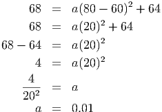
Thus, the equation of the function that seems to match the data is y = 0.01(x - 60)2 + 64, where y represents the number of motors returned, and x represents the amount of money (in thousands) spent on inspection expenditures in a given month. We should check this against a few more data points, to be certain that the function is the correct one. Since the point (75, 66) also appears to be on the function, we evaluate our candidate function at this x value to see if they match. At x = 75 our function is equal to y = 0.01(75 - 60)2 + 64 = 66.25 which is very close to the value given by the data. We don’t expect a perfect fit, because the data is not taken from an abstract function, but actually came from a real situation, so there will likely be some error in the best-fit function.