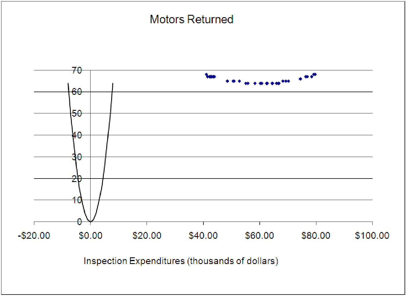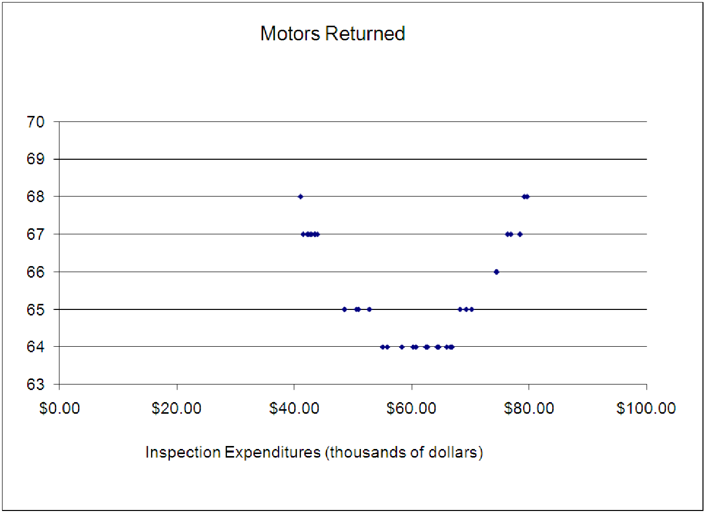
Figure 11.11: Graph of number of motors returned versus inspection expenditures.
The basic functions introduced in the last section are very useful. With these, we can fit a lot more data than we could with just straight lines. However, we often find that the data matches the shape of one of these basic functions, but not the specific location and specific points that the basic function passes through. Consider the data shown on the left scatterplot below. The data shows the number of products (in this case motors) returned from a production line as a function of the amount of money spent on inspections in a given month (in thousands of dollars). On the right is a graph of this same data, but with the graph of the basic square function superimposed on it. They have the same shape, but are not exactly the same: The square function starts too low and rises much more quickly than the actual data, and they are not in the same place on the graph.
The way to fix this is to ”move the basic function around” until it fits more closely. This is very much like what we did with straight lines before: we knew we wanted a straight line, but we needed to change the slope and y-intercept until the theoretical line matched up better with the data. For the data above, it looks like we need to ”squash” the square function down and move the starting point over and up. In this section, we’ll explore the mathematical way of doing this. When we are done, we will have developed formulas for the basic functions that are more general and contain several parameters (almost always two). These parameters are, in general, much harder to interpret than the parameters in a linear model, but once we understand how they affect the graphs, we’ll be able to out some meaning to them.