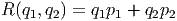
In this exploration, you will get a chance to connect the different shapes of the quadratic graphs to the values of the coefficients and see some realistic examples where these different shaped graphs might occur. Consider the revenue generated from selling two different products. Since revenue is the quantity sold (q1 will be the quantity of item 1 sold; likewise for item 2) times the unit price of the item (p1 will be the unit price of item 1) we can reasonably assume that the revenue function looks something like this:
Depending on the particular goods, we might have the prices of each item related to the quantity of both items sold. Two common situations in which this occurs are when the items are either substitute commodities, which means that people buy one or the other, but not both, or when they items are complementary commodities, where people who buy one item tend to buy the other. For example, a car company might sell one model of SUV and one model of sedan; most people buy one or the other. Thus, sedans and SUVs tend to be substitute commodities. On the other hand, since all cars need tires, we expect increased car sales to result in increased tire sales; cars and tires are complementary commodities.
We could get these relationships for the prices from the demand functions for the two items. For now, we’ll assume that the demands are linear in the prices so that:

In these expressions, the coefficients a, b, and c are all constants. The exact values of these constants depend on the relationship between the two commodities being sold.
Open the file C13 Revenue Exploration.xls [.rda] to explore how these coefficients influence the shape of the graph and the decisions that you might make in order to achieve the best possible revenue. When you open the file, depending on your computer’s security settings, you may need to click on the ”Enable Macros” button in order to make the exploration active. If all is working properly, you should have two slider bars in the upper right corner and moving these around should change the shape of the graph; if it doesn’t see the ”How To Guide” below for details on adjusting the computer’s security settings.
It is important to note that there are, potentially, six constants in the expression that you could change. We have rigged the exploration file, though, so that you can control just two of these with the slider bars, and the other four will change in a particular way. This makes it easier for you to see what is happening on the graph and allows you to focus your attention on the important features. The coefficients that you can change with the sliders are in cells C3 and D4: these represent the quantities a1 and b1 in the expressions above for the demand. You will also notice that the discriminant is calculated for you, in cell G1, to help you make some sense of what you are seeing.
Part A. First, move the sliders around to get a feel for how they interact and produce different shapes of the surface. Then concentrate on specific values of the coefficients that produce the different shapes. Finally, for one example of each shape, explain what the values of the coefficients mean in terms of the relationship between the two goods under investigation.
Now, focus on one of your graphs. The method we will use to interpret the graph is referred to as the ”method of sections”. The idea is that we fix the value of one of the independent variables; for example, we could let q2 = 500. Now we imagine moving across the surface of the graph, always keeping q2 fixed, but letting the other variable, q1 increase. The interpretation follows by thinking about what happens to the dependent variable as the free variable increases at a fixed value of the other variable (the ”sectioning variable”). For example, if you push the two sliders all the way to the right, so that cells J1 and J2 show the value of 1000, you have a graph that looks like a hill. Now, imagine setting q2 = 500 and exploring the surface along this path by letting q1 increase from 0 to 300. You might describe this exploration in the following way:
Along the section q2 = 500, the total revenue seems to be increasing until the point where q1 is about 200. Up the that point, the revenue is increasing, but at a decreasing rate (the hill is concave down). After q1 = 200, the revenue begins to decrease as q1 increases.
Similar statements can be made along any section (fixed value of one of the variables). This is very much like our interpretations of multivariable models that we have used before. The main differences are that (1) this is a graphical method and (2) we are referring to this as ”sectioning in q2” rather than ”controlling for q2” as we did in the algebraic versions.
Part B. Now, for each of the graphs you focused on in part A, describe several sections of the graph. Be sure to section the graph in both of the variables. You may want to change the viewing angle for the 3D graphs to help you visualize the surface better for some sectionings (See the How To guide for this).