When dealing with multivariable models, there are, literally, an infinite number of ways to explore them, depending on what kind of graph you want, which part of the model you want to graph, whether you would prefer looking at the data in a table of numbers, or a host of other possible choices. It helps to have some basic skills and options for visualizing functions with two independent variables. As we’ll see, graphing them requires three dimensions, one for each independent variable and one for the dependent variable. Thus, if you want to graph a model with more than two independent variables, you need some mighty special paper!
Obviously, one way to gain an understanding of how the function behaves is to make a table of data. You’ve seen such tables before for functions of several variables, you just didn’t realize it. One very common example relates to the weather. You’ve heard of wind chill probably. This is a measure of how cold the air feels, based not only on the actual temperature, but also on the wind speed. To use such a table (like the one below) you simply locate the intersection of the wind speed (down the left column) and air temperature (across the top row) to find the wind chill. Such a process defines a function of two variables. If we let W stand for the wind chill, S for wind speed and T for air temperature, then we could write
to represent the relationship; this emphasizes that W is a function of S and T. For example, W(25, 10) = -29 indicating that a 25 mph wind on a 10 degree day makes the air feel like it is actually 29 degrees below zero!
| Wind | |||||||||||||||||
| Speed | |||||||||||||||||
| (mph) | 35 | 30 | 25 | 20 | 15 | 10 | 5 | 0 | -5 | -10 | -15 | -20 | -25 | -30 | -35 | -40 | -45 |
| 5 | 33 | 27 | 21 | 16 | 12 | 7 | 1 | -6 | -11 | -15 | -20 | -26 | -31 | -35 | -41 | -47 | -54 |
| 10 | 21 | 16 | 9 | 2 | -2 | -9 | -15 | -22 | -27 | -31 | -38 | -45 | -52 | -58 | -64 | -70 | -77 |
| 15 | 16 | 11 | 1 | -6 | -11 | -18 | -25 | -33 | -40 | -45 | -51 | -60 | -65 | -70 | -78 | -85 | -90 |
| 20 | 12 | 3 | -4 | -9 | -17 | -24 | -32 | -40 | -46 | -52 | -60 | -68 | -76 | -81 | -88 | -96 | -103 |
| 25 | 7 | 0 | -7 | -15 | -22 | -29 | -37 | -45 | -52 | -58 | -67 | -75 | -83 | -89 | -96 | -104 | -112 |
| 30 | 5 | -2 | -11 | -18 | -26 | -33 | -41 | -49 | -56 | -63 | -70 | -78 | -87 | -94 | -101 | -109 | -117 |
| 35 | 3 | -4 | -13 | -20 | -27 | -35 | -43 | -52 | -60 | -67 | -72 | -83 | -90 | -98 | -105 | -113 | -123 |
| 40 | 1 | -4 | -15 | -22 | -29 | -36 | -45 | -54 | -62 | -69 | -76 | -87 | -94 | -101 | -107 | -116 | -128 |
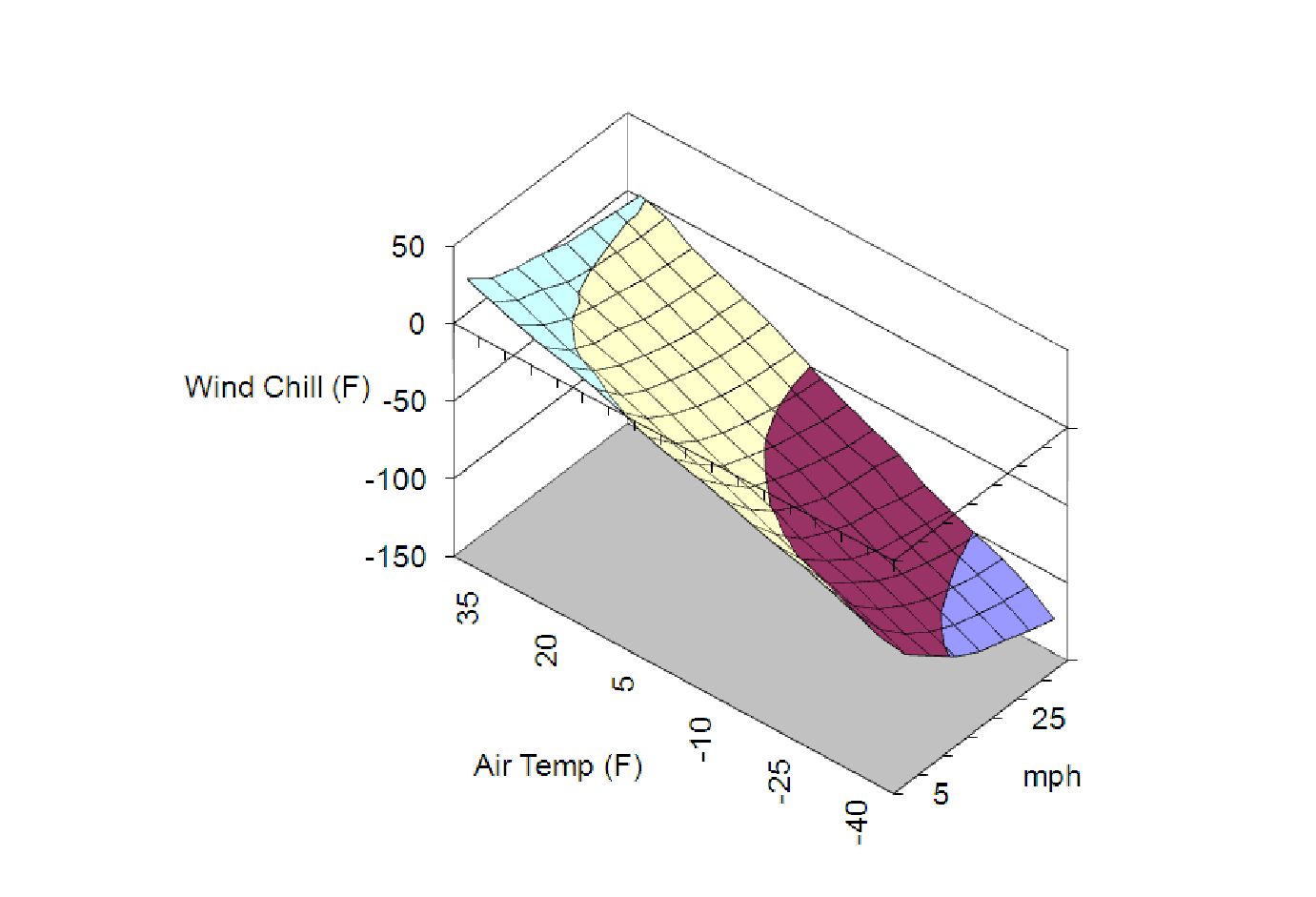
But, making tables of the data from a function is only one way to study its behavior. And, the table of numbers may be difficult to read and interpret. In addition, the spacing of the values in the table may hide some important features. For example, the wind chill table makes it appear that no matter what, if the wind speed increases, the air feels colder (wind chill is lower). But what if between 20 and 25 mph, it actually gets a little warmer for some reason? Our table would not show this.
So, another common tool for studying such functions is to create 3D surface plots of them. If we copy the table above into our spreadsheet and create such a plot, we get a figure like the one below. We can adjust the perspective of the graph, but otherwise, it has many of the same features as all the scatterplots we’ve used before.
In this section, we will use this graphical tool to help us understand the different types of quadratic models that we may get from applying the techniques of the previous section. In general, we will be dealing with models of the form

And will want to know what different shapes the graphs of such functions may take. Fortunately, there are only a few possibilities, and we will learn some ways of quickly classifying any function as being one of these types (either a bowl-shaped surface, a hill-shaped surface, or a saddle-shaped surface)
While it may seem restrictive to study such as specific class of functions, it turns out that there are several good reasons for it. The first is that it arises easily in modeling, as the techniques of the last section showed. The second is that if we zoom on the surface of any random function of two variables, on a small enough scale it looks like a quadratic. Thus, studying these objects gives us a lot of tools for understanding more complex objects.